

NCBI Bookshelf. A service of the National Library of Medicine, National Institutes of Health.
The NCBI Handbook [Internet]. 2nd edition. Bethesda (MD): National Center for Biotechnology Information (US); 2013-.
This publication is provided for historical reference only and the information may be out of date.

Scope
The NCBI Eukaryotic Genome Annotation Pipeline is an automated pipeline producing annotation of coding and non-coding genes, transcripts, and proteins on finished and unfinished public genome assemblies. It provides content for various NCBI resources including Nucleotide, Protein, BLAST, Gene, and the Map Viewer genome browser. The pipeline uses a modular framework for the execution of all annotation tasks from the fetching of raw and curated data from public repositories (sequence and Assembly databases) through the alignment of sequences and the prediction of genes, to the submission of the accessioned and named annotation products to public databases.
Core components of the pipeline are the alignment programs Splign (1) and ProSplign, and Gnomon, a gene prediction program combining information from alignments of experimental evidence and from models produced ab initio with an HMM-based algorithm.
The annotation pipeline produces comprehensive sets of genes, transcripts, and proteins derived from multiple sources, depending on the data available. In order of preference, the following sources are used:
- 1.
RefSeq curated annotated genomic sequences (2), such as the human beta globin gene cluster located on chromosome 11 (NG_000007.3)
- 2.
- 3.
Gnomon-predicted models
Both the set of genes and the placements of the genes in the annotation on the genomic sequences comprise the output of the annotation pipeline.
Organisms in scope
Those eukaryotic organisms annotated by NCBI span a wide range of taxa among invertebrates, vertebrates, and plants. Annotation priorities are based on several considerations, including:
- National Institutes of Health (NIH) priorities: Mammals are important to the NIH, so high-quality genome assemblies for new mammalian species are given a higher priority for annotation
- Biological or economic importance: highly-studied organisms or organisms with agricultural (e.g., crops) or industrial use
- Community interest/requests: requests from research communities, communicated in person or in writing through the NCBI Support Center. To write to the NCBI Support Center, click on the “Support Center” link in the bottom right corner of any NCBI web page.
The annotation process depends heavily on the availability of transcript or protein evidence for the species. Some annotation plans for high-priority organisms may be put on hold pending submission and public availability of transcriptome data.
Assemblies in scope
Only genomes with assemblies that are public in the International Nucleotide Sequence Database Collaboration (INSDC) (DNA Data Bank of Japan, European Nucleotide Archive or GenBank) are considered for annotation. These assemblies are available in the Assembly resource. Assemblies with assembled chromosomes are preferred, but assemblies made of unplaced scaffolds only may also be annotated. Assemblies for which only contigs are available are not annotated.
Assemblies with high contig and scaffold N50 are prioritized. No single quality metric is used as a strict threshold, but assemblies that have a contig N50 above 50,000 bases and/or a scaffold N50 above 2,000,000 bases are preferred, as more complete gene sets are generally produced for assemblies with higher N50 statistics. NCBI may decide not to annotate assemblies that are extremely fragmented, even if they meet other criteria.
If multiple assemblies are available for the same organism, NCBI will annotate the higher quality assembly as the reference. Alternate assemblies of lower quality may also be included. This decision depends on the quality of the alternate assemblies, their importance to the community, as well as the estimated gain from annotating extra assemblies (number of extra genes identified, compensation of low-quality regions in the reference by higher-quality regions in the alternate assembly, value to variation studies).
Some assemblies are submitted to INSDC with annotation. NCBI may elect to propagate this annotation onto RefSeq sequences. This is typically the case for model organism assemblies with well-curated annotation, such as Drosophila melanogaster (maintained by FlyBase), Saccharomyces cerevisiae (maintained by the Saccharomyces Genome Database) or Caenorhabditis elegans (maintained by WormBase) but annotation propagation from GenBank to RefSeq records may also be done for other organisms (e.g., Sorghum bicolor). For some organisms with annotation submitted to INSDC (e.g., Ailuropoda melanoleuca), NCBI may opt to annotate RefSeq copies of the assemblies, primarily to provide a more consistent RefSeq dataset across organisms of interest to the NIH.
History
NCBI’s original Eukaryotic Genome Annotation Pipeline began development in the year 2000 to annotate draft versions of the human genome assembly produced by the Human Genome Project. NCBI's annotation process has grown over the last 13 years to accommodate non-human organisms. It has also become an automated pipeline that annotates more feature types using a wider range of input data and new or improved algorithms.
In its infancy, NCBI’s Eukaryotic Genome Annotation Pipeline was a semi-manual process to annotate known genes by aligning mRNAs from GenBank and RefSeq to the genome using BLAST (3), and to generate ab initio gene model predictions in the spaces between the known genes with GenomeScan (4) guided by protein alignments. One early advance was to use EST alignments to produce model transcripts that represented EST and mRNA chains that shared introns. Another major improvement came in 2003 when Gnomon, a gene prediction program developed at NCBI based on GenScan (5), replaced GenomeScan. Gnomon allowed us to generate gene models using a combination of mRNA, EST and protein alignments as evidence, supplemented by ab initio prediction where evidence was lacking. The next major advance was the development and incorporation of splicing-aware alignment algorithms capable of placing transcripts and proteins independently while following established rules of eukaryotic splicing. NCBI's first splicing-aware transcript alignment program, Spidey (6), was developed as a research project but this program did not scale to very large data sets and it was not sufficiently robust for routine use in our annotation pipeline. Splign (1) was developed as a replacement for Spidey and was incorporated into the annotation pipeline in 2004. Splign allowed accurate placement of transcripts and aided efforts to identify problematic areas of both the genome and the transcript set. ProSplign, NCBI's splicing-aware protein alignment program, was incorporated into the annotation pipeline in 2006 to improve the accuracy of the protein-to-genomic sequence alignments used as evidence in the Gnomon gene model prediction process. In 2013, NCBI made another major enhancement to the annotation process that allowed effective use of RNA-Seq data as evidence for making transcript models. This greatly improved the quality of the annotation for many organisms that have little or no mRNA or EST data in GenBank.
As the rate that new genome assemblies deposited in GenBank increased, deficiencies in the annotation pipeline that limited our ability to scale the process beyond a small number of organisms became more apparent. In parallel to the improvements to the annotation algorithms described above, we twice re-engineered the existing process to create a new framework for parallel execution that also provides extensibility, robustness, tracking, and reproducibility. By 2009, development of the re-engineered pipeline was sufficiently advanced to switch production annotation runs from the old pipeline to the new framework. Further refinements to the process and more automation continue to improve throughput. In 2011, we annotated twice as many eukaryotic genomes as in any previous year and as of the second half of 2013 are releasing an average of 8 eukaryotic genome annotations per month.
Dataflow
Methods
Alignments
Both Splign (1) and ProSplign are global alignment tools that enable alignment of transcripts and proteins with high resolution of splice sites. The computational cost of these algorithms requires that approximate placements of the query sequences (transcripts or proteins) on the target (genome) be first identified with a local alignment tool, such as BLAST. Since a query often aligns at multiple locations, the BLAST hits are analyzed by the Compart algorithm to identify compartments prior to running Splign or ProSplign.
BLAST
See the BLAST chapter.
Compart algorithm
A compartment is defined as a sequence of compatible hits. Two BLAST hits are said to be compatible if they follow the natural flow of the target sequence. On a given strand, the relative position of the hits should be the same on both the query sequence and the genome. Compatible hits may overlap but may not be contained within one another. This definition of compatibility is transitive.
The Compart algorithm finds all non-overlapping compact compartments on the genome for a given query using a maximal coverage algorithm. Each compartment is assigned coverage, , which is a measure of how well it represents the target sequence:
In this equation is the effective length of the hit . It is usually the hit length, but if the hit overlaps with a neighbor hit, its effective length is decreased by a half of the overlap.
For cDNA alignments, where most useful hits are of very high identity, the weight equals the identity of the hit and the coverage is the number of matches. For protein alignments, the weight is a constant equal 1. In this case the coverage is simply the target sequence length covered by the hits.
When there is more than one compartment, the query sequence is covered multiple times, and to a certain extent finding all compartments is equivalent to maximization of the total coverage. In the case of exon duplication events, the additional hits should be ignored rather than turned into additional compartments. Since typically only a relatively small portion of the gene is duplicated we introduce a penalty for an additional compartment. This penalty ensures that a new compartment is created only if there is enough gene material for it. The value of this parameter is usually 25%–40% of the target sequence length. So our maximal coverage algorithm finds the compartments configuration that maximizes the following total coverage:
The process of optimization is performed very effectively using the dynamic programming algorithm.
Splign – Transcript alignment
Splign (1) is a tool for aligning spliced cDNA sequences against their genomic counterparts using pre-computed compartments. The program produces accurate spliced alignments via solving a score optimization problem formulated specifically to account for splice signals and introns.
In this formula and are the bonus for a match and the number of matches, and , are the penalty for a mismatch and the number of mismatches, and , are the penalties for opening and extending a gap. These parameters are similar to the ones used in Blastn. The introns are accounted for by introduction of a special type of gap with and as the penalties for an opening and extending an intron. The formulation discriminates between the most frequent consensus (GT/AG), less frequent consensus (GC/AG, AT/AC), and not consensus donor/acceptor sites by giving different values to .
Since the complexity of solving the global sequence alignment problem is proportional to the product of lengths of the sequences, the hits are arranged into compartments as described above and the dynamic programming matrix split into smaller blocks by seeding the global alignment with the high identity portion of the hits (Figure 1).
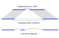
Figure 1.
Splign reduces the computational complexity by using the high identity portions of the hits (dark blue) for the bulk of the alignment and realigning only small portions of the transcript (light blue).
For each compartment, its genomic search space is expanded by the length of query cDNA ends not covered by local alignments. This allows detecting the end exons if they are missed by the local alignment tool for reasons such as the alignment length being shorter than the word size or the exon residing in a masked region. Each hit may correspond to an exon, a part of an exon, or even a number of exons. Therefore, it is important to be conservative when using local alignments for alignment seeding. Within each compartment, parts of alignments that overlap on the query are dropped. From the remaining alignments, the longest perfectly matching diagonals are extracted, and the cores are used to seed the global alignment.
Hits comprising compartments determine whether the query and the subject sequence align on the same strand. Most mRNA sequences have natural biological order and positive strand can be assumed when aligning them. On the contrary, EST and frequently RNA-Seq sequences are not oriented, so both the original sequence and its reverse complimentary have to be aligned and the strand is determined by comparing the resulting alignments.
ProSplign – Protein alignment
Protein alignments are produced by ProSplign. Similarly to Splign, ProSplign is a global protein-to-genome alignment tool that produces accurate spliced alignments from pre-computed compartments. ProSplign uses a modified Needleman Wunsch type (7) global alignment algorithm for aligning. ProSplign scores the target protein sequence against translation of the genomic sequence using the following score:
where is the score for an ungapped part of the alignment calculated using a BLOSUM62 matrix (8). Insertions and deletions for which the length is a multiple of three are scored with the default Blastp gap penalties and . Gaps for which the length is not a multiple of three are frameshifts and have a much higher opening penalty . The introns are scored as a special type of gap with a very small extension cost and an opening cost which is different between the most frequent consensus splices (GT/AG), less frequent consensus splices (GC/AG, AT/AC), and non-consensus splice sites.
Unlike Splign, ProSplign doesn’t use seeds because Blast hits for cross-species proteins do not give reliable information about seeds. Instead, ProSplign aligns the protein against a slightly extended genomic region identified by Compart as the compartment.
Not all parts of a protein are conserved well enough to provide a reliable alignment. In fact, some parts may not correspond to anything on the genome. The global alignment algorithm will align the whole protein, rendering a very low-identity alignment for the non-conserved portions of the protein. These unreliable and often misleading pieces of the alignment are filtered out by ProSplign during a post-processing step.
Gene prediction
Gnomon is a two-step gene prediction program maintained by NCBI. The Chainer algorithm assembles overlapping alignments into “chains” and is followed by the ab initio prediction step which extends these chains into complete models and creates full ab initio models, using a Hidden Markov Model (HMM).
Chainer
Spliced alignments obtained using Splign and ProSplign are likely partial, either because the aligned sequences are partial or in the case of protein alignments because only conserved portions of the protein could be aligned. Chainer analyzes and assembles these partial alignments to provide longer gene models and additional information about alternative variants.
Because of their short length and high redundancy, RNA-Seq alignments with identical introns are first combined into single alignments with larger weights (Figure 2). Boundaries of these “micro-chains” don’t cross splices known from other alignments and their extension is limited to 20 bp.
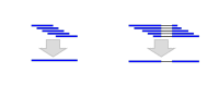
Figure 2.
Combining the alignments with the same introns into one alignment (micro chaining) reduces the computational complexity.
These “micro-chains” are then combined by Chainer with cDNA and protein alignments based on their exon structure compatibility using a modified version of the Maximal Transcript Alignment algorithm (9) based on frame compatibility of the coding regions. For protein and annotated full-length cDNA alignments, the coding regions can be inferred. For other cDNA alignments, possible coding regions are predicted and scored using a 3-periodic fifth-order Markov model for coding propensity and Weight Matrix Method (WMM) models for splice signals and translation initiation and termination signals (10). All cDNAs with coding sequence (CDS) scores above a given threshold are marked as coding, and the CDS information is used when assembling chains. In many cases, this process determines the orientation of an EST if it was unknown before. RNA-Seq and some EST alignments are too short to score above the threshold and, if they are not spliced, their orientation is often also unknown. For these alignments, Chainer will consider that these sequences can be part of the 5’ end and harbor a start codon, or be part of the 3’ end and harbor a stop codon, or be internal to the CDS or to an untranslated region (UTR), and select the scenario that contributes to the longest CDS.
Afterward, UTRs are added if the necessary translation initiation or termination signals are present. There are no restrictions on the extension of a 5’-UTR other than the exon-intron structure compatibility.
The assembled full-length chains that share splices or CDS are combined into genes with alternative isoforms. Among the partial chains for a gene, the variant with the longest CDS is selected for extension by ab initio prediction.
HMM-based prediction
The core algorithm of the ab initio prediction capability of Gnomon is based on Genscan (5), which uses a 3-periodic fifth-order HMM for the coding propensity score and incorporates descriptions of the basic transcriptional, translational and splicing signals, as well as length distributions and compositional features of exons, introns and intergenic regions. The most important distinction of Gnomon from Genscan and other ab initio prediction programs is its ability to conform to the supplied alignments and extend and complement them when necessary.
Mathematically, an HMM-based ab initio prediction is a search in the gene configuration space for the gene that provides the maximal score. If all configurations that are not compatible with the available alignments are excluded from the search space, then the optimization process in the resulting collapsed space will yield a gene configuration that is possibly suboptimal from the ab initio point of view but exactly follows the experimental information available. This approach allows extension or connections of partial alignments (Figure 3). Untranslated regions, if present in the alignments, are also included in the gene model.
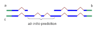
Figure 3.
Partial chains a and b produced by Chainer may be combined into one chain, c, by addition of the HMM prediction of missing coding sequence. In blue: coding sequence. In green: untranslated region
Gnomon recognizes as HMM states coding exons and introns on both strands and intergenic sequences. Translational and splice signals are described using WMM (10) and WAM (11) models. A 12-bp WMM model, beginning 6 bp prior to the initiation codon, is used for the translation initiation signal (12). A 6-bp first order WAM model starting at the stop codon is used for the translation termination signal. The donor splice signal is described by a 9-bp second order WAM model, and the acceptor splice signal is described by a 43-bp second order WAM model. Both donor and acceptor models include 3-bp of the coding exon. Coding portions of exons are modeled using an inhomogeneous 3-periodic fifth-order Markov model (13). The noncoding states are modeled using a homogeneous fifth-order Markov model.
Input data
Assemblies
The Eukaryotic Annotation Pipeline can annotate one or multiple assemblies at once (see below). All assemblies must be publicly available in the Assembly database. Since the INSDC sequence records constituting the submitted assemblies are owned by submitters and may not be modified by NCBI, all annotation is done on RefSeq copies of the INSDC assemblies. Prior to the annotation process, RefSeq accessions are assigned to the assembly’s scaffolds and chromosomes. These RefSeq sequences are based on the sequences in the INSDC records, but their records will bear the NCBI annotation. Note also that a new assembly accession, with the prefix GCF_ , is given to the assembly which contains the RefSeq sequences.
Source of evidence
The evidence used to predict gene models is selected from available public data. Same-species transcripts, proteins, and short reads, and if not sufficient, transcripts and proteins from closely related species are included.
More specifically the following sets of transcripts are included:
- Other long transcripts
- Short read RNA-Seq data available in SRA
And the following proteins:
- Known RefSeq proteins, with NP_ prefixes
- INSDC proteins derived from transcripts (as much as possible, conceptual translations are excluded)
In addition, if available for the annotated organism, curated RefSeq genomic sequences are used. These sequences have accessions with NG_ prefixes and represent non-transcribed pseudogenes, manually annotated gene clusters that are difficult to annotate via automated methods, or human RefSeqGene records (2).
Process flow
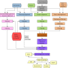
Figure 4 provides an overview of the annotation pipeline. Transcripts from RefSeq, GenBank, and the Sequence Read Archive, proteins, and, if available, RefSeq curated genomic sequences are aligned to the masked genome. Gene models are predicted by Gnomon based on these alignments, and searched against the curated database UniProtKB/SwissProt. The final set of models is then chosen among the Gnomon predictions (model RefSeq) and the known and curated RefSeq. Names and type of loci and GeneIDs are assigned to model RefSeq and retrieved from the Gene database for known RefSeq. In the final steps, the annotation is formatted, submitted to the sequences databases, and published.
Fetching of inputs
All evidence identifiers are retrieved from Entrez at the very beginning of the annotation run and the date of sequence retrieval is tracked and reported as the annotation run “freeze” date. Any sequence added to archival databases after that day will not be used.
Genome sequence masking
The assemblies are retrieved from the Assembly resource and masked using either WindowMasker (14) or RepeatMasker (15). RepeatMasker is generally used for organisms for which a comprehensive repeat library is available.
Alignment of curated RefSeq genomic sequences
If available for the organism of interest, curated RefSeq genomic sequences are aligned to the masked genome using BLAST. The alignments are ranked and filtered based on identity, coverage, and placement information kept in a RefSeq tracking in-house database. The features annotated on the alignments passing the filter are then projected onto the genomic sequences and evaluated with the other aligning evidence when choosing the best model.
Alignment of protein and transcript evidence
After retrieval, sequences are aligned to the masked genome following this general strategy: sequences are aligned locally to the genome using BLAST. Based on the BLAST hits, Compart identifies genomic compartments to which query sequences are re-aligned globally. This second round of alignments is necessary for accurate determination of splice sites and for the identification of small terminal exons that may be missed by BLAST. The global alignments are performed by Splign for transcripts and ProSplign for proteins. Resulting alignments are then ranked based on coverage and identity and filtered before hand-off to downstream tasks. Adjustments to the alignments and filtering parameters, and variation to this general dataflow are made based on the source and characteristics of the evidence and are described below.
Alignment of known RefSeq transcripts
Since many of the known RefSeq sequences are curated (most notably for Vertebrates) and, as such, are high-value targets when annotating a genome, special attention is given to their proper placement. Masking may interfere with the alignment process, so RefSeq transcripts for which all alignments on the masked genome are under a coverage threshold may be re-aligned to the unmasked genome.
The alignments are ranked and filtered based on adjustable criteria (such as coverage, identity, rank) as well as location information contained in the RefSeq tracking database. Typically, only the best-placed alignment for a given query is selected for use in downstream steps.
Alignment of non-Refseq transcripts
INSDC mRNAs, ESTs and 454 sequences are first screened against a database of mitochondrial sequences, cloning vectors, adaptors, bacterial IS-elements and repetitive sequences, and excluded from further processing if a large portion of their sequence hits a contaminant. In addition, transcripts identified as low-quality by curation staff are screened out.
Following this initial screen, the sequences are aligned with BLAST and Splign, as explained above, and ranked and filtered. For a given transcript, typically only the best-placed alignment (rank 1) is selected. For sequences that cannot be oriented (e.g., unspliced ESTs), alignments to both strands are passed dowstream. If used, cross-species transcripts are aligned with more stringent criteria than same-species transcripts to insure that only the most-likely ortholog transcript is passed downstream.
Alignment of proteins
Similarly to transcripts, proteins are first screened against a database of repeats and the curated list of low-quality transcripts. Proteins are then aligned to the masked genome with BLAST and ProSplign. The alignments are further ranked and filtered and passed to the gene prediction step.
Alignment of short reads
Short reads (RNA-Seq) available in the SRA can be used for gene prediction. A specific dataflow was engineered to handle the large volume and short length of sequences produced by new generation sequencing technologies.
RNA-Seq data from so-called next-generation sequencing platforms present several challenges for use in gene prediction. First, the reads are substantially shorter than conventional transcript data such as ESTs and mRNAs, so an individual read contains relatively little information. For example, typically only 5-25% of reads from the Illumina platform span an intron, which is the most useful data for building gene models. Second, the reads are extremely numerous and redundant, with highly-expressed genes being represented by tens of millions of reads. This presents a challenge for throughput. And third, the depth of coverage results in apparent background expression in most of the genome that isn't desirable to represent in the final gene models.
The annotation pipeline addresses these issues in several ways to reduce the complexity of the RNA-Seq data and convert it to a form useful for gene predictions:
- 1.
Datasets and associated metadata are obtained from the SRA and BioSample databases, enabling robust tracking of evidence.
- 2.
The reads are "uniquified" so that 100% identical sequences are aligned only once.
- 3.
Unique reads are aligned, ranked, and filtered for high identity and coverage alignments.
- 4.
Alignments with the same splice structure and the same or similar start and end points are collapsed into a single representative alignment. The number of reads from each SRA run is tracked for each collapsed alignment.
- 5.
Alignments containing rare introns or that represent apparent noise or background are filtered from the dataset.
Taken together, these steps reduce the size and complexity of a typical RNA-Seq dataset by 100-1000x. The resulting collapsed alignments can be used by themselves or combined with transcript and/or protein alignments for the gene prediction step.
Gene prediction by Gnomon
Protein transcript and short read alignments are passed to Gnomon for gene prediction. Chainer assembles alignments with the same exon structure and with coding regions in compatible frames into putative models. Gnomon then extends the models missing a start or a stop codon or internal exon(s) using an HMM-based algorithm. Gnomon additionally creates pure ab initio predictions where open reading frames of sufficient length but with no supporting alignment are detected (see Methods).
This first set of predictions is further refined by alignment against a subset of the nr (non-redundant) database of protein sequences. The additional alignments are added to the initial alignments and the chaining and ab initio extension steps are repeated. The results constitute the set of Gnomon predictions.
Alternate variants, complete or partial, may be produced for each gene.
Frameshifts, indels, and stop codons may occur in the resulting Gnomon predictions. They reflect sequence differences between the input transcript and protein alignments and the genome assembly.
Annotation of small RNA
tRNAs are annotated using tRNAScan-SE (16). Other small RNAs are annotated by placement of same-species curated RefSeq transcripts. Hence, these are only part of the annotation if they were incorporated in the RefSeq set for the organism being annotated. Currently the RefSeq set may include small RNAs identified by curation, collaboration, or external sources, which is currently limited to microRNAs obtained from miRBase (17).
Choosing the best model(s)
The final set of annotated features comprises, in order of preference, pre-existing known RefSeq sequences and a subset of well-supported Gnomon-predicted models. It is built by evaluating together at each locus the known RefSeq transcripts, the features projected from the curated RefSeq genomic alignments, and the models predicted by Gnomon.
Models based on known and curated RefSeq
RefSeq transcripts are given precedence over overlapping Gnomon models with the same splice pattern. Alignments of known same-species RefSeq transcripts or curated genomic sequences are used directly to annotate the gene, RNA, and CDS features on the genome. Since the RefSeq sequence may not align perfectly or completely to the genomic sequence, a consequence of this rule is that the annotated product may differ from the conceptual translation of the genome.
Models based on Gnomon predictions
Gnomon predictions are included in the final set of annotations if they do not share all splice sites with a RefSeq transcript and if they meet certain quality thresholds including:
- Only fully- or partially-supported Gnomon predictions, or pure ab initio Gnomon predictions with high coverage hits to UniProtKB/SwissProt proteins are selected.
- When multiple fully-supported transcript variants are predicted for a gene, only the Gnomon predictions supported in their entirety by a single long alignment (e.g., a full-length mRNA) or by RNA-Seq reads from a single BioSample are selected.
- Poorly-supported Gnomon predictions conflicting with better-supported models annotated on the opposite strand are excluded from the final set of models.
- Gnomon predictions with high homology to transposable or retro-transposable elements are excluded from the final set of models.
Integrating RefSeq and Gnomon annotations
As a result of the model selection process, a gene may be represented by multiple splice variants, with some of them known RefSeq and others model RefSeq (originating from Gnomon predictions).
Gnomon predictions selected for the final annotation set are assigned model RefSeq accessions with XM_ or XR_ prefixes for protein-coding and non-coding transcripts, respectively, and XP_ prefixes for proteins to distinguish them from known RefSeq with NM_/NR_ and NP_ prefixes. Model RefSeq can be searched in Entrez with the query “srcdb_refseq_model[properties]” while known RefSeq sequences can be obtained with the query “srcdb_refseq_known[properties]”.
Locus typing and protein naming
Genes are categorized into different locus types according to the type and quality of the model and based on orthology information.
- Known RefSeq features are annotated according to their locus type (e.g., protein-coding vs. pseudogene) established before the annotation run.
- Most Gnomon models with insertions, deletions, or frameshifts are labeled as pseudogenes and annotated without a CDS feature or protein product.
- Gnomon models that appear to be single-exon retrocopies of protein-coding genes may also be annotated as pseudogenes.
- Gnomon models with insertions, deletions, or frameshifts may be considered coding if they have a strong unique hit to the SwissProt database or appear to be orthologs of known protein-coding genes. Titles for these models are prefixed with “PREDICTED: LOW QUALITY PROTEIN.” There may be defects in the assembly and/or the model in these cases.
- Gnomon models that have no predicted CDS or a short CDS with no supporting alignments may be annotated as non-coding models or removed from the annotation.
- When multiple assemblies are annotated, a partial or imperfect model may be called coding because a complete model exists at the corresponding locus on one of the other annotated assemblies.
Gene and protein names are assigned based on the locus type, protein homology, and orthology information, and data from the Gene database, which may in turn be based on nomenclature from an external group such as the HUGO Gene Nomenclature Committee (HGNC). Predicted genes are evaluated for orthology to genes in a reference species using a pairwise comparison process based on protein alignments and local synteny information.
If a likely ortholog can be determined, the gene symbol and name is transferred from the reference species, if applicable.
If an ortholog cannot be determined, predicted genes are named based on the name of the most similar SwissProt protein, adding the suffix ‘-like’ to indicate the putative nature of the assignment.
Predicted genes for which no name can be determined are assigned a generic gene and protein name of the form “uncharacterized LOC” plus the GeneID.
Assignment of GeneIDs
Genes in the final set of models are assigned GeneIDs in the Gene database.
- Genes mapped from a previous annotation (see Re-annotation below) are assigned the same GeneIDs as in the previous annotation.
- Genes that are not mapped from a previous annotation and genes that are represented by Gnomon models only are assigned new GeneIDs.
- Genes mapped to equivalent locations on co-annotated assemblies are assigned the same GeneIDs (see Annotation of multiple assemblies).
Packaging of the annotation
The output of the annotation pipeline is labelled with an Annotation Release number. For a given annotation, the combination of organism and Annotation Release number (e.g., NCBI Homo sapiens Annotation Release 105) is used throughout NCBI as a way to uniquely identify annotation products originating from the same annotation run.
The annotation pipeline output is composed of the scaffolds and the chromosomes of the assembled genome(s) annotated with the genes, RNAs and proteins as features, and also the RNAs and proteins themselves. The RefSeq scaffolds and chromosomes are assigned accessions with NW_ or NT_ and NC_ prefixes and submitted to the Nucleotide database with the features annotated. Sequences submitted to the sequence databases are labelled with the Annotation Release (Figure 5).
The annotated products may include known RefSeq transcripts and proteins, Gnomon-predicted models and tRNA genes that were predicted by tRNAscan-SE. The Gnomon models that were retained by the best model selection process are submitted to the Nucleotide, Protein, and Gene database and the tRNAs genes are submitted to Gene. The known RefSeq features are updated independently from the annotation process and are not re-submitted to the sequence or Gene databases (see Access section below). The origin of the annotation can be deduced from the \note on the feature annotated on the genomic sequences (Table 1).
Table 1.
Guide to the features annotated on scaffolds and chromosomes. The note provides information on the origin of the feature. *For predicted models, the note is also on the records of individual annotation products.
For transcripts and proteins produced by Gnomon, the sequence records provide the level of support for predicted models. For low-quality proteins, the records also detail the difference between the model and the genomic sequences that was introduced to compensate for a possible error in the assembly (Figure 6).
As explained above, a known RefSeq transcript may not align perfectly to the genome but may be selected as a gene representative in the set of annotation products. These discrepancies are noted on the genomic sequence records (Figure 7).
Special considerations
Annotation of multiple assemblies
When multiple assemblies of good quality are available for a given organism, the annotation of all is done in coordination. To ensure that matching regions in multiple assemblies are annotated consistently, assemblies are mapped to each other using a BLAST-based process prior to the annotation. The reciprocal best hits are used to pair corresponding regions on two assemblies.
As explained on Figure 8, these paired regions allow the coordinate ranking of the alignment of a given transcript on both assemblies.
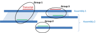
This strategy ensures that mapped regions are annotated the same way and that the same genes are assigned the same GeneID and locus type on both assemblies. It reduces the redundancy in the Gene set for a given organism and helps navigation between multiple assemblies. Note that for Gnomon models, although a single GeneID represents the locus in multiple assemblies, a different transcript and protein accession is instantiated for each individual assembly.
For more on the assembly-assembly alignment process, see the Remapping Service chapter.
Re-annotation
Special attention is given to tracking of models and genes from one release of the annotation to the next. Previous and current models annotated at overlapping genomic locations are identified and locus type and GeneID of the previous models are taken into consideration when assigning GeneIDs to the new models. If the assembly was updated between the two rounds of annotation, the assemblies are aligned to each other and the alignments used to match previous and current models in mapped regions.
Access
The status of annotation runs in progress or completed recently is updated nightly on the Eukaryotic Genome Annotation Pipeline public page:
http://www.ncbi.nlm.nih.gov/genome/annotation_euk/status/
This page provides links to the resources where data for a specific Annotation Release is available (Figure 9).
Products of NCBI’s eukaryotic annotation pipeline are available in several resources (Table 2) including:
Table 2.
Availability of annotation products in NCBI resources.
- In the Nucleotide and Protein databases
- As Map Viewer tracks
Future development: annotation reports
The quality of the end-products produced by the Eukaryotic Genome Annotation Pipeline is highly dependent on the quality of the assembly and on the amount and quality of same-species or close cross-species evidence.
To facilitate the users' understanding of the annotation process and provide context for the annotation results, NCBI will start publishing reports for each annotation run by the end of 2013. These reports will include a description of the assemblies that were annotated and summary counts of the products of the annotation. Additionally, intermediate statistics summarizing which transcripts and protein sets were used and how well the evidence aligned to the genomes will be provided.
References
- 1.
- Kapustin Y, Souvorov A, Tatusova T, Lipman D. Splign: algorithms for computing spliced alignments with identification of paralogs. Biol Direct. 2008 May 21;3:20. [PMC free article: PMC2440734] [PubMed: 18495041]
- 2.
- Pruitt KD, Tatusova T, Brown GR, Maglott DR. Nucleic Acids Res. 2012 Jan;40(Database issue):D130–5. [PMC free article: PMC3245008] [PubMed: 22121212]
- 3.
- Altschul SF, Gish W, Miller W, Myers EW, Lipman DJ. Basic local alignment search tool. J Mol Biol. 1990 Oct 5;215(3):403–10. [PubMed: 2231712]
- 4.
- Yeh RF, Lim LP, Burge CB. Computational inference of homologous gene structures in the human genome. Genome Res. 2001 May;11(5):803–816. [PMC free article: PMC311055] [PubMed: 11337476]
- 5.
- Burge C, Karlin S. Prediction of complete gene structures in human genomic DNA. J Mol Biol. 1997 Apr 25;268(1):78–94. [PubMed: 9149143]
- 6.
- Wheelan SJ, Church DM, Ostell JM. Spidey: A Tool for mRNA-to-Genomic Alignments. Genome Res. 2001 November;11(11):1952–1957. [PMC free article: PMC311166] [PubMed: 11691860]
- 7.
- Needleman SB, Wunsch CD. A general method applicable to the search for similarities in the amino acid sequence of two proteins. J Mol Bioll. 1970 Mar;48(3):443–53. [PubMed: 5420325]
- 8.
- Henikoff S, Henikoff JG. Amino acid substitution matrices from protein blocks. Proc Natl Acad Sci U S A. 1992 Nov 15;89(22):10915–9. [PMC free article: PMC50453] [PubMed: 1438297]
- 9.
- Haas BJ, Delcher AL, Mount SM, Wortman JR, Smith RK Jr, Hannick LI, Maiti R, Ronning CM, Rusch DB, Town CD, Salzberg SL, White O. Improving the Arabidopsis genome annotation using maximal transcript alignment assemblies. Nucleic Acids Res. 2003 Oct 1;31(19):5654–66. [PMC free article: PMC206470] [PubMed: 14500829]
- 10.
- Staden R. Computer methods to locate signals in nucleic acid sequences. Nucleic Acids Res. 1984 Jan 11;12(1 Pt 2):505–19. [PMC free article: PMC321067] [PubMed: 6364039]
- 11.
- Zhang MQ, Marr TG. A weight array method for splicing signal analysis. Computer applications in the biosciences. Comput Appl Biosci. 1993 Oct;9(5):499–509. [PubMed: 8293321]
- 12.
- Kozak M. Compilation and analysis of sequences upstream from the translational start site in eukaryotic mRNAs. Nucleic Acids Res. 1984 Jan 25;12(2):857–72. [PMC free article: PMC318541] [PubMed: 6694911]
- 13.
- Borodovsky M, McIninch J. GenMark: Parallel gene recognition for both DNA strands. Computers & Chemistry. 1993;17(2):123–33.
- 14.
- Morgulis A, Gertz EM, Schäffer AA, Agarwala R. WindowMasker: window-based masker for sequenced genomes. Bioinformatics. 2006 Jan 15;22(2):134-41.
- 15.
- Smit AFA, Hubley R, Green P. RepeatMasker Open-3.0. 1996–2004. http://www
.repeatmasker.org. - 16.
- Lowe TM and Eddy SR. Nucleic Acids Res. tRNAscan-SE: a program for improved detection of transfer RNA genes in genomic sequence. 1997 Mar 1;25(5):955-64. [PMC free article: PMC146525] [PubMed: 9023104]
- 17.
- Griffiths-Jones S. The microRNA Registry. Nucleic Acids Res. 2004 Jan 1;32(Database issue):D109–11. [PMC free article: PMC308757] [PubMed: 14681370]
- Eukaryotic Genome Annotation Pipeline - The NCBI HandbookEukaryotic Genome Annotation Pipeline - The NCBI Handbook
Your browsing activity is empty.
Activity recording is turned off.
See more...