NCBI Bookshelf. A service of the National Library of Medicine, National Institutes of Health.
ECRI Health Technology Assessment Group. Diagnosis and Treatment of Swallowing Disorders (Dysphagia) in Acute-Care Stroke Patients. Rockville (MD): Agency for Health Care Policy and Research (US); 1999 Jul. (Evidence Reports/Technology Assessments, No. 8.)
This publication is provided for historical reference only and the information may be out of date.

Diagnosis and Treatment of Swallowing Disorders (Dysphagia) in Acute-Care Stroke Patients.
Show detailsSensitivity and Specificity
In general, medical imaging procedures and other diagnostic tests are intended to distinguish patients with a particular condition from those without the condition. In the typical case of a binomial decision (whether the patient has the condition), there are four outcomes of the test:
- True positive (TP) (patient has condition, test detects condition)
- False negative (FN) (patient has condition, test fails to detect it)
- False positive (FP) (patient is normal, test mistakenly detects condition)
- True negative (TN) (patient is normal, test finds patient normal)
The outcomes can be expressed as a 2-by-2 table:
| Actual Condition | |||
|---|---|---|---|
| Test Results | Positive | TP | FP |
| Negative | FN | TN | |
The accuracy of the test (i.e., the fraction of results that are correct) is of only limited use in assessing the value of the test. The consequences of a false positive may be much greater or much less than the consequences of a false negative. Therefore, it is best to separately report the false-negative and false-positive rates.
FNR (false-negative rate) = FN / (TP + FN)
FPR (false-positive rate) = FP / (TN + FP)
Sensitivity and specificity (also called likelihoods) are the inverse of these quantities. They are commonly used to report results of clinical trials of a diagnostic test.
Sensitivity = the proportion of patients with the disease who are detected by the test.
Sensitivity = 1 - FNR
Sensitivity = TP / (TP + FN)
Specificity = the proportion of patients without the disease who are correctly diagnosed as negative.
Specificity = 1 - FPR
Specificity = TN / (TN + FP)
For purposes of clinical decisionmaking, it is useful to know the probability that, if a patient tests positive, the patient actually has the condition. That figure is called the positive predictive value (PPV; also called the post test probability). Its converse is the negative predictive value (NPV).
PPV = TP / (TP + FP)
NPV = TN / (TN + FN)
But the prevalence of the condition in a population other than the initial study population may be different.
Prevalence = (TP + FN) / (TP + FN + FP + TN)
If the ratio of disease positives to negatives changes, both PPV and NPV change. These parameters are not externally valid (results obtained from one patient population are not the same as results from a different patient population) so they are not usually used as the figures by which the test is judged, despite their decisionmaking significance.
The mathematical relationship between PPV and disease prevalence is described by Bayes' rule:
PPV = Sensitivity xPrevalence
(Sensitivity x Prevalence) + ((1-Specificity) x (1-Prevalence))
As prevalence increases, PPV also increases.
Sensitivity and specificity are theoretically independent of prevalence. However, sensitivity is dependent on the spectrum of severity of disease in the test population. Most diagnostic tests are more sensitive for severe disease. Also, specificity is dependent on the prevalence of comorbidities with confounding symptoms. The possibility of these types of bias should be considered whenever one examines the results of a clinical trial. Ideally, the study population of cases and controls will be selected in such a way that the prevalence of disease, spectrum of severity, and prevalence of comorbidities with confounding symptoms are the same as they would be in the population routinely examined in clinical practice.
Receiver Operating Characteristic (ROC) Analysis
Interpretation of any image or other diagnostic test requires establishing a threshold of normal variance beyond which a result will be called abnormal. This threshold may be quantitative, such as a normal limit for the concentration of something in the blood, or it may be a subjective opinion of the person interpreting the test, such as a radiologist's determination that the size and shape of the liver are not consistent with cirrhosis. Whatever the type, the threshold can be adjusted so as to increase or decrease the number of results called abnormal
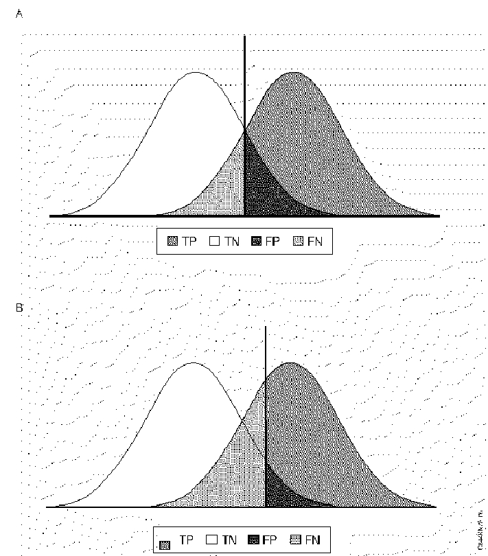
Selection of a test threshold has important effects on the sensitivity and specificity of a test and on the economic and clinical value of the test (Figure E-1 to E-4). The optimum threshold of a test may vary depending on the circumstances. For example, a preliminary screening test for HIV should have very high sensitivity because the consequences of failing to detect a person with the disease are dire. The specificity of the test is less important because all positive screening results would be confirmed with a second test. In that confirmatory test, specificity is much more important.
The relationship among sensitivity, specificity, and threshold can be described by plotting sensitivity as a function of specificity for all possible thresholds. This graph, adopted from signal detection theory, is called a receiver operating characteristic (ROC) curve. By convention, it is drawn with an inverted scale (1 - specificity) on the specificity axis. That is to say, true-positive rate is plotted as a function of false-positive rate (this is the same as a plot of the likelihood ratios at various thresholds).
The area under the ROC curve (Az) is widely considered to be a useful figure for assessing the effectiveness of a test and comparing it with that of other tests. There are a few reasons why Az is not endorsed with unanimity. First, contributions from the end of the curve are weighted equally with contributions from the center of the curve, where clinically useful thresholds are more likely to be found. Measurement of Az only within the upper left quadrant (sensitivity and specificity both more than 0.50) has been proposed as an alternative figure. Another way of summarizing the ROC into a single statistic is the partial area index, in which the area under the curve is calculated only over a clinically useful range of sensitivities. To avoid bias, that range must be selected before the meta-analysis is conducted.
Another alternative means of comparing tests using the ROC is to construct a challenge ROC using known or estimated values for the costs and benefits of each test outcome (true positive, false negative, false positive, true negative). A desired level of cost utility or net cost is chosen. For each value of specificity, the sensitivity at which the cost is exactly the chosen level is calculated. The calculated points are then connected into an ROC curve. Experimental sensitivity and specificity results for the test in question are superimposed on the graph, and it can be determined whether the test meets or does not meet the cost criteria. Finally, cost information can be used to determine an optimal operating point on the ROC, and curves can be compared at their respective optimum points.
In many situations (i.e., base case for a cost-effectiveness model), reporting of diagnostic effectiveness as a single sensitivity/specificity point is desirable. Various ways of choosing such points have been reported:
- Sensitivity at an arbitrary false-positive rate
- False-positive rate at an arbitrary sensitivity
- Sensitivity and specificity at the point where sensitivity equals specificity
- Sensitivity and specificity at the point where their sum is greatest
Each of these methods has the disadvantage of describing results at a point on the ROC curve that may be outside the range of thresholds at which the test is actually used. This is particularly bad for tests in which either sensitivity or specificity is especially valued, such as screening tests. The sensitivity/specificity at mean threshold (SMT) avoids these problems and is used in our evaluation of diagnostic tests.
Calculation of a Summary ROC
Because of the tradeoff between sensitivity and specificity, calculating an average sensitivity or specificity by averaging the sensitivity or specificity from multiple trials will underestimate the true sensitivity or specificity. For the same reasons, pooling of results from multiple trials in order to calculate a pooled sensitivity or specificity will also underestimate the true value. An exception can be made for tests that have a fixed threshold and are not subject to the interpretation of a human observer. Such tests are rare because the threshold between positive and negative results is relative and is rarely fixed absolutely, even in laboratory evaluated tests. The principle is best explained graphically. The curve in Figure 9.2 represents the sensitivity and specificity of a hypothetical test. If the results of two trials of the test (points A and B) are averaged (point M), it can be seen that the resulting mean sensitivity and specificity underestimate the value of the test.
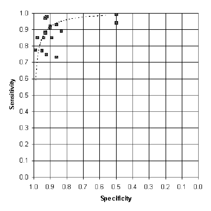
A better way to combine the results of the trials is to generate a summary ROC (SROC) curve. Littenberg and Moses (1993) have developed a linear regression method for calculation of a summary ROC. In this method, the sensitivity and specificity are transformed into a coordinate space where there is a linear relationship between sensitivity and specificity. The least-squares method can then be used to fit a straight line to the experimental results. The regression line is then back-transformed into sensitivity/specificity space to yield an SROC.
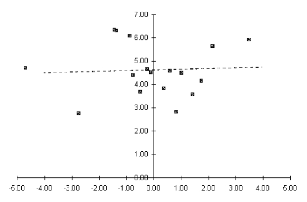
Littenberg and Moses found that logits (log odds ratios) gave the desired linear relationship necessary for the calculation. The logit of the sensitivity and specificity results of each trial is calculated according to the following equations:
logit(TPR) = ln[TPR / (1 - TPR)]
logit(FPR) = ln[FPR / (1 - FPR)]
Then parameters S and D are calculated (see equation 9-9) so that the regression will not favor TPR (true-positive rate) fitting over FPR (false-positive rate) fitting, as would be the case if the regression were to fit TPR as a function of FPR, or vice versa. S corresponds to the threshold used to distinguish between positives and negatives in a particular trial, while D corresponds to the effectiveness of the test as measured in that trial. For some tests, D may depend strongly on S.
S = logit(TPR) + logit(FPR)
D = logit(TPR) - logit(FPR)
Where sensitivity or specificity is either 0 or 1, the logit is undefined. This error arises when, due to case mix, study size, and/or test effectiveness, there is a zero value for the number of patients with results [true positive (TP), false positive (FP), false negative (FN), or true negative (TN)]. Before any such study is included in the regression, 0.5 is added to each of the categories, a correction term suggested by Littenberg and Moses. We do not add the correction term to data from studies with no zero values for TP, TN, FP, or FN. In most cases in which the correction is necessary, the zero group is either false positives or false negatives, so the effect of the correction is to very slightly underestimate the true sensitivity and specificity found in the study.
S and D are plotted (see Figure 9.3), and a straight line is fitted to them (with S defined as the independent variable and D as the dependent variable) by the least-squares method. Confidence intervals on the fitted values of D can also be calculated. The fitted line is then back-transformed into ROC space.
logit(TPR) = (S + D) / 2
logit(FPR) = (S - D)/2
sensitivity = elogit(TPR) / (1 + elogit(TPR))
specificity = 1 - [elogit(FPR) / (1 + elogit(FPR))]
Extrapolating the line beyond the maximum or minimum S values of the original data should be avoided. This prevents calculation of Az, the area under the ROC curve, which is a widely used (but sometimes criticized) measure of test effectiveness.
Experiments using simulated data have shown that the Littenberg and Moses method gives a close approximation to real ROC curves. Without a priori knowledge of the form of the curve, it is impossible to know what the true fit is. Actual ROC data for different tests fit different curve forms, but the logit regression method is an accepted compromise.
To obtain the sensitivity/specificity at mean threshold, we averaged the S values for all trials in the meta-analysis. The corresponding value of D was calculated from the regression equations, and the logit-space (S, D) point was back-transformed into ROC space (sensitivity, specificity) to yield sensitivity/specificity at mean threshold. This mean threshold method is an objective way to select one clinically relevant or typical data point from an SROC curve to use as a base case in decision analysis.
For this technology assessment, regression calculations were carried out using the SPSS statistical software system (version 6.1 for Windows, SPSS Inc., Chicago, Illinois). Results from the SPSS system were transferred to an Excel spreadsheet (Microsoft Corp., Redmond, Washington) for plotting and to allow comparison of one set of results with another.
Figure E-1. Threshold Effects in Diagnosis
 The left peak represents the frequency distribution of the nondiseased population, and the right peak represents the diseased population. The value of the phenomenon measured by the diagnostic test increases horizontally from left to right. The vertical line represents the threshold value. In B specificity has been increased by raising the threshold, which decreases the number of false positives, but which decreases sensitivity and increases the number of false negatives.
Figure E-2. Mean Sensitivity and Specificity are Not Accurate

Figure E-3. Logit Transform of Sensitivity/specificity Results

Figure E-4. Regression Line Transformed into ROC Space
 The outer X marks on these summary ROC plots represent the minimum and maximum thresholds observed in the clinical trials going into the summary ROC. Portions on the curve beyond these thresholds are extrapolations; these sensitivities and specificities may not be attainable in clinical practice.
The X in the center of each curve represents the sensitivity and specificity at the mean threshold. This point is the one best estimate of the sensitivity and specificity of the test.
- Appendix E. Methods for Evaluation of Diagnostic Tests - Diagnosis and Treatment...Appendix E. Methods for Evaluation of Diagnostic Tests - Diagnosis and Treatment of Swallowing Disorders (Dysphagia) in Acute-Care Stroke Patients
Your browsing activity is empty.
Activity recording is turned off.
See more...