

NCBI Bookshelf. A service of the National Library of Medicine, National Institutes of Health.
McEntyre J, Ostell J, editors. The NCBI Handbook [Internet]. Bethesda (MD): National Center for Biotechnology Information (US); 2002-.

This publication is provided for historical reference only and the information may be out of date.

Summary
Sequence variations exist at defined positions within genomes and are responsible for individual phenotypic characteristics, including a person's propensity toward complex disorders such as heart disease and cancer. As tools for understanding human variation and molecular genetics, sequence variations can be used for gene mapping, definition of population structure, and performance of functional studies.
The Single Nucleotide Polymorphism database (dbSNP) is a public-domain archive for a broad collection of simple genetic polymorphisms. This collection of polymorphisms includes single-base nucleotide substitutions (also known as single nucleotide polymorphisms or SNPs), small-scale multi-base deletions or insertions (also called deletion insertion polymorphisms or DIPs), and retroposable element insertions and microsatellite repeat variations (also called short tandem repeats or STRs). Please note that in this chapter, you can substitute any class of variation for the term SNP. Each dbSNP entry includes the sequence context of the polymorphism (i.e., the surrounding sequence), the occurrence frequency of the polymorphism (by population or individual), and the experimental method(s), protocols, and conditions used to assay the variation.
dbSNP accepts submissions for variations in any species and from any part of a genome. This document will provide you with options for finding SNPs in dbSNP, discuss dbSNP content and organization, and furnish instructions to help you create your own (local) copy of dbSNP.
Introduction
The dbSNP has been designed to support submissions and research into a broad range of biological problems. These include physical mapping, functional analysis, pharmacogenomics, association studies, and evolutionary studies. Because dbSNP was developed to complement GenBank, it may contain nucleotide sequences (Figure 1) from any organism.
Physical Mapping
In the physical mapping of nucleotide sequences, variations are used as positional markers. When mapped to a unique location in a genome, variation markers work with the same logic as Sequence Tagged Sites (STSs) or framework microsatellite markers. As is the case for STSs, the position of a variation is defined by its unique flanking sequence, and hence, variations can serve as stable landmarks in the genome, even if the variation is fixed for one allele in a sample. When multiple alleles are observed in a sample pedigree, pedigree members can be tested for variation genotypes as in traditional physical mapping studies.
Functional Analysis
Variations that occur in functional regions of genes or in conserved non-coding regions might cause significant changes in the complement of transcribed sequences. This can lead to changes in protein expression that can affect aspects of the phenotype such as metabolism or cell signaling. We note possible functional implications of DNA sequence variations in dbSNP in terms of how the variation alters mRNA transcripts.
Association Studies
The associations between variations and complex genetic traits are more ambiguous than simple, single-gene mutations that lead to a phenotypic change. When multiple genes are involved in a trait, then the identification of the genetic causes of the trait requires the identification of the chromosomal segment combinations, or haplotypes, that carry the putative gene variants.
Evolutionary Studies
The variations in dbSNP currently represent an uneven but large sampling of genome diversity. The human data in dbSNP include submissions from the SNP Consortium, variations mined from genome sequence as part of the human genome project, and individual lab contributions of variations in specific genes, mRNAs, ESTs, or genomic regions.
Null Results Are Important
Systematic surveys of sequence variation will undoubtedly reveal sequences that are invariant in the sample. These observations can be submitted to dbSNP as NoVariation records that record the sequence, the population, and the sample size that were used in the survey.
Searching dbSNP
The SNP database can be queried from the dbSNP homepage (Figures 2a and 2b), by using Entrez SNP, or by using the links to the six basic dbSNP search options located just below the text box at the top of the dbSNP homepage. Each of these six search options is described below.
Figure
Figure 2a. We organized the dbSNP homepage with links to documentation, FTP, and sub-query pages on the left sidebar and a selection of query modules on the right sidebar.
Figure
Figure 2b. We organized the dbSNP homepage with links to documentation, FTP, and sub-query pages on the left sidebar and a selection of query modules on the right sidebar.
Entrez SNP
dbSNP is a part of the Entrez integrated information retrieval system (Chapter 15) and may be searched using either qualifiers (aliases) or a combination of 25 different search fields. A complete list of the qualifiers and search fields can be found on the Entrez SNP site.
Single Record (Search by ID Number) Query in dbSNP
Use this query module to select SNPs based on dbSNP record identifiers. These include reference SNP (refSNP) cluster ID numbers (rs#), submitted SNP Accession numbers (ss#), local (or submitter) IDs, Celera IDs, Genbank accession numbers, and STS accession numbers.
SNP Submission Information Queries
Use this module to construct a query that will select SNPs based on submission records by laboratory (submitter), new data (called “new batches” — this query limitation is more recent than a user-specified date), the methods used to assay for variation (Table 1) populations of interest (Table 2), and publication information.
Table
Table 1. Method classes organize submissions by a general methodological or experimental approach to assaying for variation in the DNA sequence.
Table
Table 2. Population classes organize population samples by geographic region.
dbSNP Batch Query
Use sets of variation IDs (including RefSNP (rs) IDs, Submitted SNP (ss) IDs, and Local SNP IDs) collected from other queries to generate a variety of SNP reports.
Locus Information Query
This search was originally accomplished by LocusLink, which has now been replaced by Entrez Gene. Entrez Gene is the successor to LocusLink and has two major differences that differentiate it from Locus Link: Entrez Gene is greater in scope (more of the genomes represented by NCBI Reference Sequences or RefSeqs) and Entrez Gene has been integrated for indexing and query in NCBI's Entrez system.
Between-Markers Positional Query
Use this query approach if you are interested in retrieving variations that have been mapped to a specific region of the genome bounded by two STS markers. Other map-based queries are available through the NCBI Map Viewer tool.
ADA Section 508-compliant Link
All links located on the left sidebar of the dbSNP homepage are also provided in text format at the bottom of the page to support browsing by text-based Web browsers. Suggestions for improving database access by disabled persons should be sent to the dbSNP development group at snp-admin@ncbi.nlm.nih.gov.
Submitted Content
The SNP database has two major classes of content: the first class is submitted data, i.e., original observations of sequence variation; and the second class is computed content, i.e., content generated during the dbSNP “build” cycle by computation on original submitted data. Computed content consists of refSNPs, other computed data, and links that increase the utility of dbSNP.
A complete copy of the SNP database is publicly available and can be downloaded from the SNP FTP site (see the section How to Create a Local Copy of dbSNP). dbSNP accepts submissions from public laboratories and private organizations. (There are online instructions for preparing a submission to dbSNP.) A short tag or abbreviation called Submitter HANDLE uniquely defines each submitting laboratory and groups the submissions within the database. The 10 major data elements of a submission follow.
Flanking Sequence Context DNA or cDNA
The essential component of a submission to dbSNP is the nucleotide sequence itself. dbSNP accepts submissions as either genomic DNA or cDNA (i.e., sequenced mRNA transcript) sequence. Sequence submissions have a minimum length requirement to maximize the specificity of the sequence in larger contexts, such as a reference genome sequence. We also structure submissions so that the user can distinguish regions of sequence actually surveyed for variation from regions of sequence that are cut and pasted from a published reference sequence to satisfy the minimum-length requirements. Figure 1 shows the details of flanking sequence structure.
Alleles
Alleles define variation class (Table 3). In the dbSNP submission scheme, we define single-nucleotide variants as G, A, T, or C. We do not permit ambiguous IUPAC codes, such as N, in the allele definition of a variation. In cases where variants occur in close proximity to one another, we permit IUPAC codes such as N, and in the flanking sequence of a variation, we actually encourage them. See Table 3 for the rules that guide dbSNP post-submission processing in assigning allele classes to each variation.
Table
Table 3. Allele definitions define the class of the variation in dbSNP.
Method
Each submitter defines the methods in their submission as either the techniques used to assay variation or the techniques used to estimate allele frequencies. We group methods by method class (Table 1) to facilitate queries using general experimental technique as a query field. The submitter provides all other details of the techniques in a free-text description of the method. Submitters can also use the METHOD_EXCEPTION_ field to describe changes to a general protocol for particular sets of data (batch-specific details). Submitters generally define methods only once in the database.
Population
Each submitter defines population samples either as the group used to initially identify variations or as the group used to identify population-specific measures of allele frequencies. These populations may be one and the same in some experimental designs. We assign populations a population class (Table 2) based on the geographic origin of the sample. These broad categories provide a general framework for organizing the approximately 700 (as of this writing) sample descriptions in dbSNP. Similar to method descriptions, population descriptions minimally require the submitter to provide a Population ID and a free-text description of the sample.
Sample Size
There are two sample-size fields in dbSNP. One field is called SNPASSAY SAMPLE SIZE, and it reports the number of chromosomes in the sample used to initially ascertain or discover the variation. The other sample size field is called SNPPOPUSE SAMPLE SIZE, and it reports the number of chromosomes used as the denominator in computing estimates of allele frequencies. These two measures need not be the same.
Population-specific Allele Frequencies
Alleles typically exist at different frequencies in different populations; a very common allele in one population may be quite rare in another population. Also, allelic variants can emerge as private polymorphisms when particular populations have been reproductively isolated from neighboring groups, as is the case with religious isolates or island populations. Frequency data are submitted to dbSNP as allele counts or binned frequency intervals, depending on the precision of the experimental method used to make the measurement. dbSNP contains records of allele frequencies for specific population samples defined by each submitter (Table 4).
Table
Table 4. Validation status codes summarize the available validation data in assay reports and refSNP clusters.
Population-specific Genotype Frequencies
Similar to alleles, genotypes have frequencies in populations that can be submitted to dbSNP.
Population-specific Heterozygosity Estimates
Some methods for detection of variation (e.g., denaturing high-pressure liquid chromatography or DHPLC) can recognize when DNA fragments contain a variation without resolving the precise nature of the sequence change. These data define an empirical measure of heterozygosity when submitted to dbSNP.
Individual Genotypes
dbSNP accepts individual genotypes for samples from publicly available repositories such as CEPH or Coriell. Genotypes reported in dbSNP contain links to population and method descriptions. General genotype data provide the foundation for individual haplotype definitions and are useful for selecting positive and negative control reagents in new experiments.
Validation Information
dbSNP accepts individual assay records (ss numbers) without validation evidence. When possible, however, we try to distinguish high-quality validated data from unconfirmed (usually computational) variation reports. Assays validated directly by the submitter through the VALIDATION section show the type of evidence used to confirm the variation. Additionally, dbSNP will flag an assay as validated (Table 4) when we observe frequency or genotype data for the record.
Computed Content (The dbSNP Build Cycle)
We release the content of dbSNP to the public in periodic “builds” that we synchronize with the release of new genome assemblies for each organism (Chapter 14). During each build, we map both the data submitted since the last build and the current refSNP set to the genome. The following 7 tasks define the sequence of steps in the dbSNP build cycle (Figure 3).
Submitted SNPs and Reference SNP Clusters
Once a new SNP is submitted to dbSNP, it is assigned a unique submitted SNP ID number (ss#). Once the ss number is assigned, we align the flanking sequence of each submitted SNP to its appropriate genomic contig. If several ss numbers map to the same position on the contig, we cluster them together, call the cluster a “reference SNP cluster”, or “refSNP”, and provide the cluster with a unique RefSNP ID number (rs#). If only one ss number maps to a specific position, then that ss is assigned an rs number and is the only member of its RefSNP cluster until another submitted SNP is found that maps to the same position.
A refSNP has a number of summary properties that are computed over all cluster members (Figure 4), and are used to annotate the variations contained in other NCBI resources. We export the entire dbSNP refSNP set in many report formats on the FTP site, and deliver them as sets of results when a user conducts a dbSNP batch query. We also maintain both refSNPs and submitted SNPs in FASTA databases for use in BLAST searches of dbSNP.
New Submissions and the Start of a New Build
Each build starts with a “close of data” that defines the set of new submissions that will be mapped to genome sequence by multiple cycles of BLAST and MegaBLAST for subsequent annotation and grouping of the SNPs into refSNPs. The set of new data entering each build typically includes all submissions received since the close of data in the previous build.
Mapping to a Genome Sequence
When a new genome build is ready, dbSNP obtains the FASTA files for submitted SNPs that were submitted prior to the “close of data”, as well as the FASTA files for the refSNPs in the current build, and then maps the submitted SNPs and refSNPs to the genome sequence using the procedure described in Appendix 2. The refSNP set is also mapped to the previous genome assembly to support users who require older mapping data (e.g. during the production cycle for dbSNP human build 126, The refSNP set was mapped to both human build 36.1 and human build 35.1).
It should also be mentioned that during a build cycle, some organisms have refSNPs mapped to multiple assemblies (e.g. human has two major assemblies: the NCBI Reference Genome assembly and the Celera assembly).
refSNP Clustering and refSNP Orientation
Since submitters to dbSNP can arbitrarily define variations on either strand of DNA sequence, submissions in a refSNP cluster can be reported on the forward or reverse strand. The orientation of the refSNP, and hence its sequence and allele string, is set by a cluster exemplar. By convention, the cluster exemplar is the member of a cluster that has longest sequence. In subsequent builds, this sequence may be in reverse orientation to the current orientation of the refSNP. When this occurs, we preserve the orientation of the refSNP by using the reverse complement of the cluster exemplar to set the orientation of the refSNP sequence.
Once the clustering process determines the orientation of all member sequences in a cluster, it will gather a comprehensive set of alleles for a refSNP cluster.
| Hint: |
|---|
| When the alleles of a submission appear to be different from the alleles of its parent refSNP, check the orientation of the submission for reverse orientation. |
Re-Mapping and refSNP Merging
RefSNPs are operationally defined as a variation at a location on an ideal reference chromosome. Such reference chromosomes are the goal of genome assemblies. However, since work is still in progress on many of the genome projects, and since even the‘finished’ genomes are updated to correct past annotation errors, we currently define a refSNP as a variation in the interim reference sequence. Every time there is a genomic assembly update, the interim reference sequence may change, so the refSNPs must be updated or re-clustered.
The re-clustering process begins when NCBI updates the genomic assembly. All existing refSNPs (rs) and newly submitted SNPs (ss) are mapped to the genome assembly using multiple BLAST and MegaBLAST cycles as delineated in Appendix 2. We then cluster SNPs that co-locate at the same place on the genome into a single refSNP. Newly submitted SNPs can either co-locate to form a new refSNP cluster, or may instead cluster with an already existing refSNP. When newly submitted SNPs cluster among themselves, they are assigned a new refSNP number, and when they cluster with an already existing refSNP, they are assigned to that refSNP cluster.
Sometimes an existing refSNP will co-locate with another refSNP when dbSNP begins using an improved clustering algorithm, or when genome assemblies change between builds. A refSNP co-locates with another refSNP only if the mapped chromosome positions of the two refSNPs are identical. So when dbSNP uses an improved clustering algorithm that enhances our ability to more precisely place refSNPs, if the new placement of a refSNP is identical in location to another refSNP, the two refSNPs co-locate. Similarly, if a change in a genome assembly alters the position of a refSNP so that it is identical with the position of another refSNP, the two refSNPs co-locate. When two existing refSNPs co-locate, the refSNP with the higher refSNP number is retired (which means we never reuse it), and all the submitted SNPs in that higher refSNP cluster number are re-assigned to the refSNP with the lower refSNP number. The re-assignment of the submitted SNPs from a higher refSNP number to a refSNP cluster with a lower refSNP number is called a “merge”, and occurs during the “rs merge” step of the dbSNP mapping process. Merging is only used to reduce redundancy in the catalog of rs numbers so that each position has a unique identifier. All "rs merge" actions that occur are recorded and tracked.
There is an important exception to the merge process described above; this exception occurs when a co-locating SNP meets certain clinical and publication criteria. A refSNP meeting these criteria is termed “precious” and will keep its original refSNP number (the refSNP number will NOT retire as discussed above) if it co-locates with a SNP that has a lower refSNP number. The purpose of having “precious” SNPs is to maintain refSNP number continuity for those SNPs that have been cited in the literature and are clinically important.
Once the clusters are formed, the variation of a refSNP is the union of all possible alleles defined in the set of submitted SNPs that compose the cluster.
Please Note: dbSNP only merges rs numbers that have an identical set of mappings to a genome and the same allele type (e.g. both must be the same variation type and share one allele in common). We therefore would not merge a SNP and an indel (insertion/deletion) into a single rs number (different variation classes) since they represent two different types of mutational "events".
RefSNP Number Stability
The stability of a refSNP number depends on what is meant by “stable”. If a refSNP number has been merged into another refSNP number, it is very easy to use a retired refSNP number to find the current refSNP number (see hint below) — so in this case, one could consider a refSNP number to be stable since merged refSNP numbers are always associated with, and can always retrieve the current refSNP number.
| Hint: |
|---|
There are three ways the you can locate the partner numbers of a merged refSNP:
|
If, however, what is meant by “stable” is that the refSNP number of a particular variation always remains the same, then one should not consider a refSNP entirely stable, as a refSNP number may change if two refSNP numbers merge as described above. Merging is more likely to happen, however, if the submitted flanking sequence of the refSNP exemplar is short, is of low quality, or if the genome assembly is immature. A refSNP number may also change if:
- dbSNP breaks up an existing cluster and re-instantiates a retired rs number based on a reported conflict from a dbSNP user (a less than 1 in 1,000,000 occurrence)
Functional Analysis
Variation Functional Class
We compute a functional context for sequence variations by inspecting the flanking sequence for gene features during the contig annotation process, and do the same for RefSeq/GenBank mRNAs.
Table 5 defines variation functional classes. We base class on the relationship between a variation and any local gene features. If a variation is near a transcript or in a transcript interval, but not in the coding region, then we define the functional class by the position of the variation relative to the structure of the aligned transcript. In other words, a variation may be near a gene (locus region), in a UTR (mRNA-utr), in an intron (intron), or in a splice site (splice site). If the variation is in a coding region, then the functional class of the variation depends on how each allele may affect the translated peptide sequence.
Table
Table 5. Function codes for refSNPs in gene features. a
Typically, one allele of a variation will be the same as the contig (contig reference), and the other allele will be either a synonymous change or a non-synonymous change. In some cases, one allele will be a synonymous change, and the other allele will be a non-synonymous change. If either allele in the variation is a non-synonymous change, then the variation is classified as non-synonymous; otherwise, the variation is classified as a synonymous variation. The primary functional classifications are as follows:
- The functional class is noted as coding when a problem with the annotated coding region feature prohibits conceptual translation. The coding notation is based solely on position in this case.
Because functional classification is defined by positional and sequence parameters, two facts emerge: (a) if a gene has multiple transcripts because of alternative splicing, then a variation may have several different functional relationships to the gene; and (b) if multiple genes are densely packed in a contig region, then a variation at a single location in the genome may have multiple, potentially different, relationships to its local gene neighbors.
SNP Position in 3D Structure
When a SNP results in amino acid sequence change, knowing where that amino acid lies in the protein structure is valuable. We provide this information using the following procedure: To find the location of a SNP within a particular protein, we attempt to identify similar proteins whose structure is known by comparing the protein sequence against proteins from the PDB database of known protein structures using BLAST. Then, if we find matches, we use the BLAST alignment to identify the amino acid in the protein of known structure that corresponds to the amino acid containing the SNP. We store the position of the amino acid on the 3D structure that corresponds to the amino acid containing the SNP in the dbSNP table SNP3D.
Population Diversity Data
The best single measure of a variation's diversity in different populations is its average heterozygosity. This measure serves as the general probability that both alleles are in a diploid individual or in a sample of two chromosomes. Estimates of average heterozygosity have an accompanying standard error based on the sample sizes of the underlying data, which reflects the overall uncertainty of the estimate. dbSNP’s computation of average heterozygosity and standard error for RefSNP clusters is available online. Please note that dbSNP computes heterozygosity based on the submitted allele frequency for each SNP. If the frequency data for a SNP is not submitted, we cannot compute the heterozygosity value, and therefore the refSNP report will show no heterozygosity estimate.
Additional population diversity data include population counts, individuals sampled for a variation, genotype frequencies, and Hardy Weinberg probabilities.
Build Resource Integration
We annotate the non-redundant set of variations (refSNP cluster set) on reference genome sequence contigs, chromosomes, mRNAs, and proteins as part of the NCBI RefSeq project (Chapter 18). We compute summary properties for each refSNP cluster, which we then use to build fresh indexes for dbSNP in the Entrez databases, and to update the variation map in the NCBI Map Viewer. Finally, we update links between dbSNP and dbMHC, OMIM, Homologene, the NCBI Probe database, PubMed, UniGene, and UniSTS.
Annotating GenBank and Other RefSeq Records
GenBank records can be annotated only by their original authors. Therefore, when we find high-quality hits of refSNP records to the HTGS and non-redundant divisions of GenBank, we connect them using LinkOut (Chapter 17).
We annotate RefSeq mRNAs with variation features when the refSNP has a high-quality hit to the mRNA sequence. If the variation is in the coding region of the transcript and has a non-synonymous allele that changes the protein sequence, we also annotate the variation on the protein translation of the mRNA. The alleles in protein annotations are the amino acid translations of the affected codons.
NCBI Map Viewer Variation and Linkage Maps
The Map Viewer (Chapter 20) can show multiple maps of sequence features in common chromosome coordinates. The variation map shows all variation features that we annotate on the current genome assembly. There are two ways to see the variation data. The default graphic mode shows the data as tick marks on the vertical coordinate scale. When variation is selected as the master map from the Maps and Options drop-down menu, and the user zooms in on the map to the individual RefSNP level, a summary of map quality, variation quality warning, functional relationships to genes, average heterozygosity with standard error, and validation information are provided. If genotype, haplotype, or LinkOut data are available, the master map will also contain links to this information.
Public Release
Public release of a new build involves an update to the public database and the production of a new set of files on the dbSNP FTP site. We make an announcement to the dbsnp-announce mailing list when the new build for an organism is publicly available.
dbSNP Resource Integration
Links from SNP Records to Submitter Websites
The SNP database supports and encourages connections between assay records (submitted SNP ID numbers, or ss numbers) and supplementary data on the submitter's Web site. This connection is made using the LINKOUT field in the SNPassay batch header. LinkOut URLs are base URLs to which dbSNP can append the submitter's ID for the variation to construct a complete URL to the specific data for the record. We provide LinkOut pointers in the batch header section of SNP detail reports and in the refSNP report cluster membership section.
Links within NCBI
We make the following connections between refSNP clusters and other NCBI resources during the contig annotation process:
Entrez Gene
There are two methods by which we localize variations to known genes: (a) if a variation is mapped to the genome, we note the variation/gene relationship (Table 5) during functional classification and store the locus_id of the gene in the dbSNP table SNPContigLocusId; and (b) if the variation does not map to the genome, we look for high-quality blast hits for the variation against mRNA sequence. We note these hits with the protein_ID (PID) of the protein (the conceptual translation of the mRNA transcript). Entrez Gene scans this table nightly and updates the table MapLinkPID with the locus_id for the gene when the protein is a known product of a gene.
UniSTS
When an original submitted SNP record shows a relationship between a SNP and a STS, we share the data with dbSTS and establish a link between the SNP and the STS record. We also examine refSNPs for proximity to STS features during contig annotation. When we determine that a variation needs to be placed within an STS feature, we note the relationship in the dbSNP table SnpInSts.
UniGene
The contig annotation pipeline relates refSNPs to UniGene EST clusters based on shared chromosomal location. We store Variation/UniGene cluster relationships in the dbSNP table UnigeneSnp.
PubMed
We connect individual submissions to PubMed record(s) of publications cited at the time of submission. To view links from PubMed to dbSNP, select “linkouts” as a PubMed query result.
dbMHC
dbSNP stores the underlying variation data that define HLA alleles at the nucleotide level. The combinations of alleles that define specific HLA alleles are stored in dbMHC. dbSNP points to dbMHC at the haplotype level, and dbMHC points to dbSNP at both the haplotype and variation level.
How to Create a Local Copy of dbSNP
dbSNP is a relational database that contains hundreds of tables. Since the inception of build 125, the design dbSNP has been altered to a ”hub and spoke” model, where the dbSNP_Main_Table acts as the hub of a wheel, storing all of the central tables of the database, while each spoke of the wheel is an organism-specific database that contains the latest data for a specific organism. dbSNP exports the full contents of the database for the public to download from the dbSNP FTP site.
Due to security concerns and vendor endorsement issues, we cannot provide users with direct dumps of dbSNP. The task of creating a local copy of dbSNP can be complicated, and should be left to an experienced programmer. The following sections will guide you in the process of creating a local copy of dbSNP, but these instructions assume knowledge of relational databases, and were not written with the novice in mind.
If you have problems establishing a local copy of dbSNP, please contact dbSNP at snp-admin@ncbi.nlm.nih.gov.
Schema: The dbSNP Physical Model
A schema is a necessary part of constructing your own copy of dbSNP because it is a visual representation of dbSNP that shows the logical relationship between data in dbSNP. It is available as a printable PDF file from the dbSNP FTP site.
Data in dbSNP are organized into “subject areas” depending on the nature of the data. The data dictionary currently includes a description of all the tables in dbSNP as well as tables of columns and their properties. Foreign keys are not enforced in the physical model because they make it harder to load table data asynchronously. In the future, we will add descriptions of individual columns. The data dictionary is also available online from the dbSNP Web site.
Resources Required for Creating a Local Copy of dbSNP
Software:
- Relational database software. If you are planning to create a local copy of dbSNP, you must first have a relational database server, such as Sybase, Microsoft SQL server, or Oracle. dbSNP at NCBI runs on an MSSQL server version 2000, but we know of users who have successfully created their local copy of dbSNP on Oracle.
Hardware:
- Computer platforms/OS. Databases can be maintained on any PC, Mac, or UNIX with an Internet connection.
- Disk space. Currently, a complete copy of dbSNP that will include all organisms contained in dbSNP requires 500 GB of space. Depending on the organism you are interested in, you can simply create a local database that only includes data for the organism of your interest. Please allow room for growth.
- Memory. The current sql server for dbSNP has 4GB of memory.
- Internet connection. We recommend a high-speed connection to download such large database files.
dbSNP Data Location
The FTP database directory in the dbSNP FTP site contains the schema, data, and SQL statements to create the tables and indices for dbSNP:
- The shared_schema subdirectory contains the schema DDL (SQL Data Definition Language) for the dbSNP_main_table.
- The shared_data subdirectory contains data housed in the dbSNP_main_table that is shared by all organisms.
- The organism_schema sub-directory contains links to the schema DDL for each organism specific database.
- The organism_data sub-directory contains links to the data housed in each organism specific database. The data organized in tables, where there is one file per table. The file name convention is: <tablename>.bcp.gz. The file name convention for the mapping table also includes the dbSNP build ID number and the NCBI genome build ID number. For example, B125_SNPContigLoc_35_1 means that during dbSNP build 125, this SNPContigLoc table has SNPs mapped to NCBI contig build 35 version 1. The data files have one line per table row. Fields of data within each file are tab delimited.
dbSNP uses standard SQL DDL(Data Definition Language) to create tables, views for those tables, and indexes. There are many utilities available to generate table/index creation statements from a database.
| Hint |
|---|
| If your firewall blocks passive FTP, you might get an error message that reads: “Passive mode refused. Turning off passive mode. No control connection for command: No such file or directory”. If this happens, try using a "smart" FTP client like NCFTP (available on most UNIX machines). Smart FTP clients are better at auto-negotiating active/passive FTP connections than are older FTP clients (e.g. Sun Solaris FTP). |
Stepwise Procedure for Creating a Local Copy of dbSNP
- 1.
Prepare the local area.
(check available space, etc.)
- 2.
Download the schema files.
- a.
Download the following files from the dbSNP shared
_schema sub-directory: dbSNP_main_table, dbSNP_main_index_constraint, and all the files in the shared _data sub-directory. Together, the files from both of these sub-directories will allow you to create tables and indices for the dbSNP_main_table.
- b.
Go to the organism
_schema subdirectory, and select the organism for which you wish to create a database. For the purpose of this example, human_9606 has been selected. Once human_9606 is selected, you will be directed to the human organism_schema sub-directory. Download all of the files contained in this subdirectory.
- c.
Go to the organism
_data subdirectory, and select the organism for which you wish to create a database. For the purpose of this example, human_9606 has been selected. Once you select human_9606, you will be directed to the human organism_data sub-directory. Download all of the files contained in this subdirectory.
A user must always down load the files located in the most recent versions of the shared_schema and shared_data sub-directories in addition to any organism specific content.
Save all the files in your local directory and decompress them.
| Hint: |
|---|
| On a UNIX operating system, use gunzip to decompress the files: dbSNP_main_table and dbSNP_main_index_constraint. The files on the SNP FTP site are UNIX files. UNIX, MS-DOS and Macintosh text files use different characters to indicate a new line. Load the appropriate new line conversion program for your system before using bcp. |
- 3.
Create the dbSNP_main_table
- a.
From the shared
_schema sub-directory, use the dbSNP_main_table file to create tables, and use the dbSNP_main_index_constraint files to create indices for the dbSNP main database.
- b.
Load all of the bcp files located in the shared
_data sub-directory into the dbSNP_main_table you just created using the data-loading tool of your database server (e.g., bcp for Sybase). See the sample FTP protocol and sample Unix C Shell script (below) for directions.
- c.
Create indices by opening the dbSNP_main_index_constraint.sql file. If you are using a database server that provides the isql utility, then use the following command:
isql -S <servername> -U usename -P password -i dbSNP_main_index_constraint.sql
- 4.
Create the organism specific database
Once the dbSNP_main_table has been created, create the organism specific database using the files in your specific organism’s organism_schema and organism_data subdirectories. Human_9606 will be used for the purpose of this example:
- a.
Create the human_9606 database using the following files found in the human_9606 organism
_schema: human_9606_table.sql.gz, human_9606_view.sql.gz, human_9606_index_constraint.sql.gz,
and human_9606_foreign_key.sql.gz
- b.
Load all of the bcp files located in the shared
_data sub-directory into the human_9606 database you just created using the data-loading tool of your database server (e.g., bcp for Sybase). See the sample FTP protocol and sample Unix C shell script (below) for directions.
| Hint: |
|---|
| Use “ftp -i” to turn off interactive prompting during multiple file transfers to avoid having to hit “yes” to confirm transfer hundreds of times. |
| Hint: |
|---|
| To avoid an overflow of your transaction log while using the bcp command option (available in Sybase and SQL servers), select the "batch mode" by using the command option: -b number of rows. For example, the command option -b 10000 will cause a commit to the table every 10,000 rows. |
- 5.
Sample FTP Loading protocol.
- a.
Type ftp -i ftp.ncbi.nih.gov (Use "anonymous" as user name and your email as your password).
- b.
Type: cd snp/database
- c.
To get dbSNP_main for shared tables and shared data: Type ls to see if you are in the directory with the right files. Then type “cd shared_schema” to get schema file for dbSNP_main, and finally, type “cd shared_data” to get the data for dbSNP_main.
- d.
Type binary (to set binary transfer mode).
- e.
Type mget *.gz (to initiate transfer). Depending on the speed of the connection, this may take hours since the total transfer size is gigabytes in size and growing.
- f.
To decompress the *.gz files, type gunzip *.gz. (Currently, the total size of the uncompressed bcp files is over 10 GB).
- 6.
Use scripts to automate data loading.
- a.
Located in the loadscript subdirectory of the dbSNP FTP site, there is a file called cmd.create_local_dbSNP.txt that provides a sample UNIX C shell script for creating a local copy of dbSNP_main and a local copy of a specific organism database using files in the shared_schema, and the organism_schema sub-directories.
- b.
Also in the the loadscript subdirectory of the dbSNP FTP site, there is a file called cmd.bulkinsert.txt that provides a sample UNIX C shell script for loading tables with files located in shared_data and organism_data sub-directories.
- 7.
Data integrity (creating a partial local copy of dbSNP).
dbSNP is a relational database. Each table has either a unique index or a primary key. Foreign keys are not reinforced. There are advantages and a disadvantage to this approach. The advantages are that this approach makes it easy to drop and re-create the table using the dbSNP_main_table, which then makes it possible to create a partial local copy of dbSNP. For example, if you are interested only in the original submitted SNP and their population frequencies, and not in their map locations on NCBI genome contigs or GenBank Accession numbers (both are huge tables), then these tables can be skipped (i.e., SNPContigLoc and MapLink). Please remember that mapping tables such as SNPContigLoc will have a build ID prefix and suffix included in its file name. (e.g. SNPContigLoc will be b125_SNPContigLoc_35_1for SNP build 125, and NCBI contig build 35 version 1). Of course, to select tables for a particular query, the contents of each table and the dbSNP entity relationship (ER) diagram need to be understood. The disadvantage of un-reinforced references is that either the stored procedures or the external code needs to be written to ensure the referential integrity.
Appendix 1. dbSNP report formats.
ASN.1
The docsum_2005.asn file is the ASN structure definition file for ASN.1 and is located in the /specs subdirectory of the dbSNP FTP site. The 00readme file, located in the main dbSNP FTP directory, provides information about ASN.1 data structure and data exchange. ASN.1 text or binary output can be converted into one or more of the following formats: flatfile, FASTA, docsum, chromosome report, RS/SS, and XML. To convert from ASN.1 to another format, request ASN.1 output from either the dbSNP FTP site or the dbSNP batch query pages, and use dstool (located in the “bin” directory of the dSNP FTP site) to locally convert the output into as many alternative formats as needed.
XML
The XML format provides query-specific information about refSNP clusters,
as well as cluster members in the NCBI SNP Exchange (NSE) format. The XML schema is located in the docsum_2005.xsd file, which is housed in the /specs sub-directory of the dbSNP FTP site. A human-readable text form of the NSE definitions can be found in docsum_2005.asn, also located in the /specs sub-directory of the dbSNP FTP site.
FASTA: ss and rs
The FASTA report format provides the flanking sequence for each report of variation in dbSNP, as well as all the submitted sequences that have no variation. ss FASTA contains all submitted SNP sequences in FASTA format, whereas rs FASTA contains all the reference SNP sequences in FASTA format. The FASTA data format is typically used for sequence comparisons using BLAST. BLAST SNP is useful for conducting a few sequence comparisons in the FASTA format, whereas multiple FASTA sequence comparisons will require the construction of a local BLAST database of FASTA formatted data and the installation of a local stand-alone version of BLAST.
rs docsum Flatfile
The rs docsum flatfile report is generated from the ASN.1 datafiles and is provided in the files "/ASN1_flat/ds_flat_chXX.flat". Files are generated per chromosome (chXX in file name),as with all of the large report dumps. Because flatfile reports are compact, they will not provide you with as much information as the ASN.1 binary report, but they are useful for scanning human SNP data manually because they provide detailed information at a glance. A full description of the information provided in the rs docsum flatfile format is available in the 00readme file, located in the SNP directory of the SNP FTP site.
Chromosome Reports
The chromosome reports format provides an ordered list of RefSNPs in approximate chromosome coordinates. Chromosome reports is a small file to download but contains a great deal of information that might be helpful in identifying SNPs useful as markers on maps or contigs because the coordinate system used in this format is the same as that used for the NCBI genome Map Viewer. It should also be mentioned that the chromosome reports directory might contain the multi/ file and/or the noton/ files. These files are lists (in chromosome report format) of SNPs that hit multiple chromosomes in the genome and those that did not hit any chromosomes in the genome, respectively. A full description of the information provided in the chromosome reports format is available in the 00readme file, located in the SNP directory of the SNP FTP site.
Genotype Report
The dbSNP Genotype report shows strain-specific genotype information for model organisms, and contains a genotype detail link as well as a genotype XML link. The genotype detail link will provide the user with submitter and genotype information for each of the submitted SNPs in a refSNP cluster of interest, and the genotype XML link will allow the user to download the reported data in the Genotype Exchange XML format, which can be read by either Internet Explorer or Netscape browsers. XML dumps via the dbSNP ftp server provide the same content for all genotype data in dbSNP by organism and chromosome.
Appendix 2. Rules and methodology for mapping
A cycle of MegaBLAST and Blast alignment to the NCBI genome assembly of an organism is initiated either by the appearance of FASTA-formatted genome sequence for a new build of the assembly or by the significant accrual of newly submitted SNP data for that organism.
Organism-specific Genome Mapping
The refSNP(rs) and submitted SNP (ss) mapping process is a multi-step, computer-based procedure that begins when refSNP and submitted SNP FASTA sets are aligned to the most recent genome assembly using BLAST or MegaBLAST. Repeat masking during this process is accomplished automatically using the BLAST/MegaBLAST “Dust” option. To increase alignment stringency, multiple cycles of BLAST/MegaBLAST are employed, where the word size limit is reduced from 64 in the first cycle to16 by the final cycle. MegaBLAST parameters are set to a default position with the exception of a seeding hit suppression parameter(e.g. Parameter="-U F -F 'mL' -J T -X 10 -r 1 -q -3 -W 64 -m 11 -e 0.01")that suppresses seeding hits but allows extension through regions of lowercase sequence. The quality of each alignment is determined using an Alignment Profiling Function developed specifically for this purpose. Alignments are selected based on a variable stringency threshold that ranges from 70% alignment to 50% alignment. If the alignment profiling function indicates the quality of the alignment is below a 70% alignment threshold, the alignment is discarded, although an alignment threshold of 50% is sometimes used in case there are gaps in the sequence.
The BLAST/MegaBLAST output of ASN.1 binary files of local alignments is then analyzed by an algorithm (“Globalizer”) that sorts those local alignments that do not fit the dbSNP alignment profile criteria (defined by position and proximity to one another) to create a “Global Alignment” — a group of local alignments that lay close to one another on a sequence. If the global alignment is greater than or equal to a pre-determined percentage of the flanking sequence, it is accepted as a true alignment between the refSNP or submitted SNP and the genome assembly. The Globalizer is especially helpful when refSNPs or submitted SNPs based on mRNA sequence are being aligned to the genome assembly. In such a case, the MegaBLAST/BLAST ASN.1 binary output contains many small alignments that will not map to the genome assembly unless they undergo the “globalization” process.
The ASN.1 binary output of “Globalizer” is then processed by a program called “Hit Analyzer”. This program defines the alleles and LOC types for each hit, and also determines the map position by using the closest map positions on either side of the SNP to establish the hit location. The text output of “Hit Analyzer” is then processed by the “Hit Filter”, which filters out paralogous hits and uses multiple strategies to select only those SNPs that have the greatest degree of alignment to a particular contig. The output from the “Hit Filter” is then placed into a map.bcp file and is processed by the “SnpMapInfo” program, which creates an MD5 signature for each SNP that is representative of all the positional information available for that SNP. The MD5 signature is then placed in the SNP MAP INFO file, which is then loaded into dbSNP.
RefSNPs and submitted SNPs are analyzed against GenBank mRNA, RefSeq mRNA, and GenBank clone accessions using a similar procedure to that described in the above paragraphs.
Once the all the results from previous steps are loaded into dbSNP, we perform cluster analysis using a program called “SNPHitCluster” which analyses SNPs having the same signatures to find candidates for clustering. If an MD5 signature for a particular SNP is different from the MD5 signature of another SNP, then the hits for those two SNPs are different, and therefore, the SNPs are unique and need not be clustered. If an MD5 signature of a particular SNP is the same as that of another SNP, the two SNPs may have the same hit pattern, and if after further analysis, the hit patterns are shown to be the same, the two SNPs will be clustered.
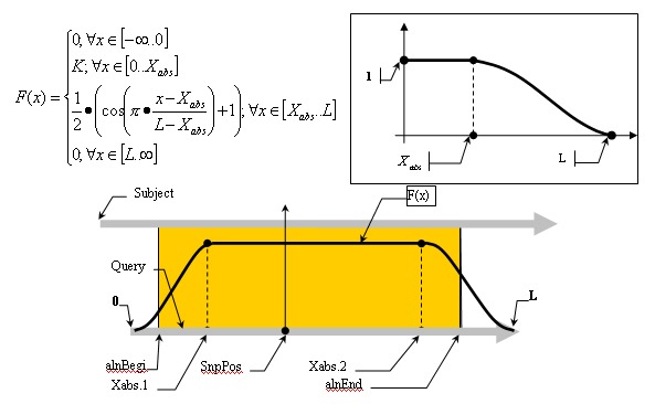
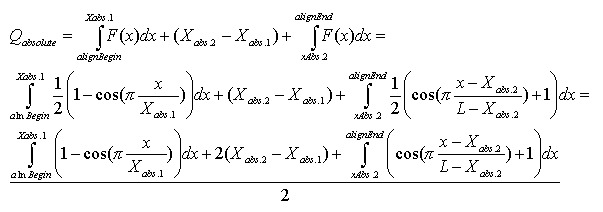
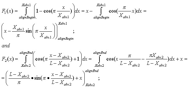
Appendix 3 Alignment profiling function
Mismatch weights are not equal along the flanking sequence, and should therefore be assigned according to a profiling function. Because of the nature of the sequencing process, it is common to have errors concentrated along the flanking sequence tails; we must, therefore, be mindful of this consideration and not disregard alignments in the tails of the query sequence just because of the high concentration of errors found there. Let us assume, therefore, that the distribution of errors follows the rule of natural distribution starting on some point within the flank. This can be approximated with the function F(x):
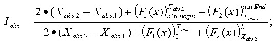
Alignment Quality, “Q”, can be calculated using the following equation:
Having:
The optimistic identity rate (so named since it doesn’t include mismatches) can be calculated by the following function:
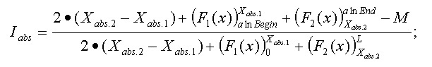
Mismatches will affect the numerator of the above function. A function to describe mismatches will contain parts of unmovable discontinuations. Strictly speaking, we must take the integral of this function in order to determine the mismatch effect, but due to the corpuscular nature of the alignment, we can easily replace it with the sum of the elementary function:
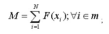
where m is the mismatch position vector.
Thus, the final function:
Appendix 4. 3D structure neighbor analysis.
When a protein is known to have a structure neighbor, dbSNP projects the RefSNPs located in that protein sequence onto sequence structures.
First, contig annotation results provide the SNP ID (snp_id), protein accession (protein_acc), contig and SNP amino acid residue (residue), as well as the amino acid position (aa_position) for a particular RefSNP. These data can be found in the dbSNP table, SNPContigLocusId. FASTA sequence is then obtained for each protein accession using the program idfetch, with the command line parameters set to:
-t 5 -dp -c 1 -q
We BLAST these sequences against the PDB database using “blastall” with the command line parameters set to:
-p blastp -d pdb -i protein.fasta -o result.blast -e 0.0001 -m 3 -I T -v 1 -b 1
Each SNP position in the protein sequence is used to determine its corresponding amino acid and amino acid position in the 3D structure from the BLAST result. These data are stored in the SNP3D table.
- Summary
- Introduction
- Searching dbSNP
- Submitted Content
- Computed Content (The dbSNP Build Cycle)
- dbSNP Resource Integration
- How to Create a Local Copy of dbSNP
- Appendix 1. dbSNP report formats.
- Appendix 2. Rules and methodology for mapping
- Appendix 3 Alignment profiling function
- Appendix 4. 3D structure neighbor analysis.
- The Single Nucleotide Polymorphism Database (dbSNP) of Nucleotide Sequence Varia...The Single Nucleotide Polymorphism Database (dbSNP) of Nucleotide Sequence Variation - The NCBI Handbook
Your browsing activity is empty.
Activity recording is turned off.
See more...