NCBI Bookshelf. A service of the National Library of Medicine, National Institutes of Health.
McEntyre J, Ostell J, editors. The NCBI Handbook [Internet]. Bethesda (MD): National Center for Biotechnology Information (US); 2002-.

This publication is provided for historical reference only and the information may be out of date.
Summary
The primary data produced by genome sequencing projects are often highly fragmented and sparsely annotated. This is especially true for the Human Genome Project as a result of its policy of releasing sequence data to the public sequence databases every day (1, 2). So that individual researchers do not have to piece together extended segments of a genome and then relate the sequence to genetic maps and known genes, NCBI provides annotated assemblies of public genome sequence data. NCBI assimilates data of various types, from numerous sources, to provide an integrated view of a genome, making it easier for researchers to spot informative relationships that might not have been apparent from looking at the primary data. The annotated genomes can be explored using Map Viewer (Chapter 20) to display different types of data side-by-side and to follow links between related pieces of data.
This chapter describes the series of steps, the “pipeline”, that produces NCBI's annotated genome assembly from data deposited in the public sequence databases. A variant of the annotation process developed for the human genome is used to annotate the mouse genome, and similar procedures will be applied to other genomes (Box 1).
NCBI constantly strives to improve the accuracy of its human genome assembly and annotation, to make the data displays more informative, and to enhance the utility of our access tools. Each run through the assembly and annotation procedure, together with feedback from outside groups and individual users, is used to improve the process, refine the parameters for individual steps, and add new features. Consequently, the details of the assembly and annotation process change from one run to the next. This chapter, therefore, describes the overall human genome assembly and annotation process and provides short descriptions of the key steps, but it does not detail specific procedures or parameters. However, sufficient detail is provided to enable users of our assembly and annotations to become familiar with the complexities and possible limitations of the data we provide.
Overview of the Genome Assembly and Annotation Process
Figure 1 shows how the main steps in the human genome assembly and annotation process are organized and also shows the most significant interdependencies between the steps. The pipeline is not linear, because whenever possible, steps are performed in parallel to reduce the overall time taken to produce an annotated assembly from a new set of data. Some of the steps are run incrementally on a timetable that is independent from that of the main pipeline to produce a new assembly more quickly.
Data Freeze
New sequence data that could be used to improve the genome assembly and annotation become available on a daily basis. Since the assembly and annotation process takes several weeks to complete, the data are “frozen” at the start of the build process by making a copy of all of the data available for use at that time. Freezing the data provides a stable set of inputs for the remainder of the build process. Additional or revised data that become available during the period taken to complete the process are not used until the next build.
The Build Cycle
A build begins with a freeze of the input data and ends with the public release of an annotated assembly of genomic sequences (Figure 1). There are usually a few months between builds so that the latest build can be evaluated and improvements can be made.
Steps Run Incrementally
The early steps of the genome assembly and annotation pipeline involve many computationally intensive processes, including masking the repetitive sequences and aligning each genomic sequence to the other genomic sequences, mRNAs, and Expressed Sequence Tags (ESTs). Running these steps incrementally minimizes the time between starting a new build and being ready to start the assembly and annotation steps. Approximately once a week, independent from the build cycle, new or updated sequences that have been deposited in GenBank are retrieved for processing. Periodically, old versions of the sequences are purged from the set of accumulated data files.
The manual refinement of the set of assembled genomic contigs produced entirely from finished sequence is another time-consuming step that is carried out incrementally, approximately once a week.
Steps Run Irregularly
Because some data change infrequently, some relatively quick steps are executed on time frames that are not tied to the build cycle. For example, the list of special cases used to override the automatic process is updated whenever the need becomes apparent.
The Input Data
The main inputs for the genome assembly and annotation process are genomic sequences, transcript sequences, and Sequence Tagged Site (STS) maps.
Human Genomic Sequences
Genomic Sequences Used for Assembly
Genomic sequences from the following five data sets are processed for use in the assembly:
High-Throughput Genomic Sequences. Human high-throughput genomic sequences (HTGSs) are retrieved using the Entrez query system (Chapter 15). The query used returns sequences for all entries that contain the HTG keyword, regardless of whether the sequence is finished or is in any of the unfinished draft phases.
Finished Chromosome Sequences. The center that coordinates the sequencing of a finished chromosome submits a specification regarding how to build the sequence of that chromosome from its component clone sequences to a data repository at the European Bioinformatics Institute (EBI). The sequences specified for any finished chromosomes are retrieved from GenBank and included in the set of genomic sequences to be processed for an assembly.
Genomic Sequences from the Tiling Paths of Individual Chromosomes. The human genome sequencing centers use a variety of experimental evidence to compile an ordered list of clones they believe provides the best coverage for each chromosome. At least once every 2 months, the sequencing centers submit an updated minimal tiling path for each chromosome to a data repository at the EBI. These tiling path files (TPFs) include Accession numbers if sequence for a clone is available. The tiling path repository is checked each day for the Accession numbers from any tiling path that has been updated. Any secondary Accession numbers are replaced with the corresponding primary Accession numbers, and any invalid Accession numbers are flagged to prevent those sequences from being used for assembly. The latest version of the sequence for each Accession number in the most recent clone tiling paths is retrieved from GenBank and included in the set of genomic sequences to be processed for assembly.
Assembled Blocks of Contiguous Finished Genomic Sequence. As the sequences for individual clones are finished, they are merged with overlapping finished sequences to form contigs (3). The primary source for identifying neighboring clones is the clone tiling path for each chromosome. Additional information is obtained from some GenBank entries that contain annotation specifying the neighboring clones. BLAST (4) is used to align the sequences of candidate pairs of clones, and a merged sequence is produced automatically if the expected overlap is confirmed by the sequence alignment. When the automatic processes do not find an expected overlap, there is a manual review to find the correct overlap, refining the clone order if necessary. The most recent set of finished contigs are processed for assembly.
Additional Genomic Sequences. A few other specific human genomic sequences are added to the assembly set because they contain genes that may not be represented in the genomic sequences from the other sources.
Genomic Sequences Used for Ordering and Orienting
Sequences known to come from both ends of the same cloned genomic fragment provide valuable linking information that helps to order and orient sequence contigs in the assembly step (5, 6). The SNP Consortium sequenced the ends of the inserts in several million plasmid clones containing small (0.8–6 Kbp) fragments of human genomic DNA. In many cases, both ends of the same insert were sequenced (Table 4 in Ref. 7), thereby providing a set of plasmid paired-end sequences.
Genomic Sequences Used for Annotation
Curated Genomic Regions. The Reference Sequence project (Chapter 18; Refs. 8, 9) provides reviewed annotated sequences for a number of genomic regions that are difficult to annotate correctly by automated processes (e.g., immunoglobulin gene regions). These Reference Sequences (RefSeqs) are aligned to the assembled genome so that the curated annotation can be transferred to the assembled genomic sequence. RefSeqs for known pseudogenes are also aligned, not only to enable transfer of the correct annotation but, more importantly, to prevent prediction of erroneous model transcripts and proteins.
BAC End Sequences. Sequences from the ends of human genomic inserts in Bacterial Artificial Chromosome (BAC) clones are used to help map the location of specific clones onto the assembled genome sequence. The BAC end sequences are obtained from dbGSS (see Chapter 1). The clone names are extracted and converted to a standardized format to facilitate linking of the BAC end sequences with mapping data and additional sequences for the same clone, when these are available.
Genomic Sequences Used for Alignment
Human genomic sequences that are not used for either assembly or annotation are processed so that their relationships to the assembled genome can be displayed in Map Viewer (Chapter 20). Most genomic sequences deposited in GenBank by individual scientists will not be HTG and therefore will not be used for assembly; however, they are used for alignment. The exceptions are a few non-HTG sequences that are used for assembly, because they are included in the clone tiling path of an individual chromosome or in an assembled block of finished sequence. Any sequences intended for assembly but not used, either because they are redundant or are rejected by one of the quality screens in the assembly process, are also used for alignment.
Human Transcript Sequences
Human transcript sequences are used to help order and orient genomic fragments in the assembly step, for feature annotation and also to produce maps that show the locations of the transcripts on the assembled genome. Transcripts used include: (a) human mRNA RefSeqs (8, 9), except model transcripts produced from previous rounds of genome annotation; (b) human mRNA sequences deposited in GenBank by individual scientists, except those mRNAs produced after a translocation or other rearrangement of the genome; and (c) a nonredundant set of EST sequences from the BLAST FTP site. Additional information relating to these EST sequences is obtained from UniGene (Chapter 21).
Transcripts from Other Organisms
Transcripts from other organisms may be aligned to the genome being processed. These data may reveal the location of potential genes not identified by other means. RefSeq mRNAs, GenBank mRNAs, and ESTs, obtained from the same sources that provide the human transcripts, are used. Their alignments are processed for display in Map Viewer but are not used in the assembly step or for feature annotation.
Sequence Tagged Site (STS) Maps
Genetic linkage maps, radiation hybrid (RH) maps, and a YAC map are used to help avoid assembling genomic contigs incorrectly and to help place the contigs along the chromosomes. The positions of STS markers on various maps (Table 1) are transformed into a common format that allows us to compare the maps to each other during the assembly process. Additional maps are processed so that they can be displayed in Map Viewer.
The maps listed in Table 1 are static and are not updated with additional markers. Any new STS maps are added to our data set soon after they are released.
Special Cases
Our own review of previous genome assemblies or feedback from users sometimes identify particular cases in which bad data or overlooked data prevent the automated processes from producing the best possible assembly of a particular segment of the genome. To help guide the assembly process, a list of such special cases is maintained. The list is used to provide supplemental data that override the automatic processes that assign a particular input genomic sequence to a chromosome or determine whether it is used for assembly.
Preparation of the Input Sequences
The raw input genomic sequences are screened for contaminants, the repetitive sequences are masked, and the draft genomic sequences are split into fragments in preparation for alignment to other sequences. The input transcript sequences are also screened for contaminants before they are aligned to the genomic sequences. The STS content of the input genomic sequences is determined.
Preparation of Genomic Sequences
Removing Contaminants
Draft-quality HTGSs sometimes contain segments of sequence derived from foreign sources, most commonly the cloning vector or bacterial host. Finished sequences are usually, but not always, free of such contaminants. Common contaminants introduce artificial blocks of homologous sequence that can give rise to misleading alignments between two unrelated genomic sequences. MegaBLAST (10) is used to compare the raw genomic sequences to a database of contaminant sequences (including the UniVec database of vector sequences, the Escherichia coli genome, bacterial insertion sequences, and bacteriophage). Any foreign segments are removed from draft-quality sequence or masked in finished sequence to prevent them from participating in alignments.
Masking of Repetitive Sequences
Sequences that occur in many copies in the genome will align to many different clones. Such repetitive sequences include interspersed repeats (SINEs, LINEs, LTR elements, and DNA transposons), satellite sequences, and low-complexity sequences (7, 11, 12). Matches between repetitive sequences on unrelated clones make it difficult to identify alignments that indicate a genuine overlap between clones. To eliminate the confounding matches that are based only on repetitive sequences, the genomic sequences are run through RepeatMasker to identify known repeats. Repeats are masked by converting the sequence to lowercase letters so that they do not initiate alignments.
Fragmentation of Draft Sequences
Draft HTGSs consist of a set of sequence contigs derived from a particular clone artificially linked together to form a single sequence. The masked, draft genomic sequences are split at the gaps between their constituent contigs to create separate sequence fragments that can be aligned independently. Vector sequences and other contaminants are also removed at this stage by trimming or further splitting the sequence fragments.
Determination of STS Content
Any STS markers contained within the input genomic sequences are identified by e-PCR (13) using the UniSTS database. The resulting data are used primarily to relate the genomic sequences to independently derived STS maps (genetic, radiation hybrid) but are also used to identify some foreign sequences.
Filtering
Sequences from other clones being sequenced at the same institution can occasionally cross-contaminate draft HTGSs. The contaminating sequences may come from another clone from the same organism or from another organism. The raw genomic sequences are screened in several ways to detect cross-contamination: (a) they are compared with the genome sequences from completely sequenced organisms using MegaBLAST (10); (b) they are screened for the presence of organism-specific interspersed repeats using RepeatMasker; and (3) they are screened for the presence of mapped STS markers from other organisms using e-PCR (13). Any input sequence that contains foreign sequences, repeats, or markers is flagged for removal from the data set used for assembly. Draft sequences longer than the maximum insert length expected for a genomic clone are also rejected because it is likely they are contaminated with sequences from at least one other clone.
At this stage, draft sequences composed of fragments that are too small to contribute significantly to the assembly or that are tagged with the HTGS_CANCELLED keyword are also flagged for removal. Another filter rejects sequences annotated as being from another organism or as being RNA, erroneously included in the input sequences.
Chromosome Assignment
To improve assembly of the genomic sequences, the input genomic sequences are assigned to a specific chromosome before attempting to merge the sequences. Genomic sequences that appear on any of the chromosome tiling paths are automatically assigned to the designated chromosome. Other genomic sequences are assigned to a chromosome based on: (a) annotation on the submitted GenBank record; (b) the presence of multiple STS markers that have been mapped to the same chromosome; (c) fluorescence in situ hybridization (FISH) mapping (14, 15); or (d) personal communication from a scientist with specialized knowledge. If there is no assignment, or the assignments are conflicted, the sequences are treated as unassigned and assembled without constraint by chromosome.
Filtering of Transcript Sequences
Transcript sequences that contain sequences derived from vectors or other common contaminants can produce artificial alignments to the assembled genomic sequence. The input transcript sequences are therefore compared with a database of contaminants using MegaBLAST (10), as described for genomic sequences. Any transcripts with significant matches to the sequence of a contaminant are excluded from the set of transcript sequences used for genome assembly or annotation.
mRNA sequences shorter than 300 bases are excluded from the set of sequences that are aligned to the genomic sequences because they are too small to contribute significantly to genome assembly or annotation. Also excluded are any mRNA sequences flagged because they do not represent the true sequence of a transcript, e.g., those that are chimeric or contain genomic sequences.
Alignment of Sequences to the Input Genomic Sequences
Alignment of the input genomic sequences to each other and to various other sequences is essential for both genome assembly and genome annotation. All relevant sequences are initially aligned to the unassembled genomic sequences because this means that the computationally intensive alignment processes can be run incrementally at an early stage in the pipeline. If necessary, these alignments are remapped to the sequence of the assembled genome at a later stage by a process that requires relatively little computation.
Alignment of Genomic Sequences to Each Other
Assembly of the genomic sequences from individual clones into longer contiguous sequences (contigs) requires knowledge of which sequences overlap. The overlaps between genomic sequences are evaluated by aligning the sequences from individual genomic clones to each other. After masking of repeats, decontamination and fragmentation, each fragment of genomic sequence is aligned pairwise to all of the other fragments using MegaBLAST (10). Alignments that are sufficiently long and of sufficiently high percentage identity are saved for consideration in the assembly step.
Alignment of Clone End Sequences to the Genomic Sequences
The pairs of short genomic sequences derived from the ends of plasmid clones help to order and orient sequence fragments in the assembly step. These clone end sequences are aligned to the processed genomic sequences, as described for Alignment of Genomic Sequences to Each Other.
Alignment of Transcripts to the Genomic Sequences
Annotation of genes requires knowledge of where the sequences for known transcripts align to the assembled genomic sequences. RefSeq RNA sequences, mRNA sequences from GenBank, and EST sequences from dbEST are aligned to the processed genomic sequences, as described for Alignment of Genomic Sequences to Each Other. Later, the alignments are remapped to the assembled genomic sequence.
Alignment of Curated Genomic Regions to the Genomic Sequences
Curated genomic regions provide accurate annotation for regions of the genome that are difficult to annotate correctly by automated processes. Sequences from curated genomic regions are initially aligned to the unassembled genomic sequences and later remapped to the sequence of the assembled genome, as described for Alignment of Transcripts to the Genomic Sequences.
Alignment of Translated Genomic Sequences to Proteins
Homologies between the polypeptides encoded by the genomic sequences and known proteins/conserved protein domains provide hints for the gene prediction process. The repeat-masked genomic sequences are compared with a non-redundant database of vertebrate proteins and to the NCBI Conserved Domain Database (CDD; Ref. 16) using different versions of BLAST (4) (BLASTX and RPS-BLAST, respectively). Significant alignments are saved for use in the gene prediction step.
Genome Assembly
The input genomic sequences are assembled into a series of genomic sequence contigs. These are then ordered, oriented with respect to each other, and placed along each chromosome with appropriately sized gaps inserted between adjacent contigs. The resulting genome assembly thus consists of a set of genomic sequence contigs and a specification for how to arrange the sequence contigs along each chromosome.
Finished Chromosomes
A chromosome sequence is considered finished when any gaps that remain cannot be closed using current cloning and sequencing technology. In practice, therefore, the sequence for a finished chromosome usually consists of a small number of genomic sequence contigs. These are assembled from their component clone sequences according to the specification provided by the center responsible for sequencing that chromosome. This specification also prescribes the order, orientation, and estimated sizes for the gaps between contigs.
Unfinished Chromosomes
Genomic sequence contigs for unfinished chromosomes are assembled and laid out based largely on the clone tiling path. However, the tiling paths do not specify the orientation of the clone sequences or how they should be joined; therefore, data on the alignment of the input genomic sequences to each other and to other sequences are also used to guide the assembly. Genomic sequences that augment the initial set of genomic contigs based on the tiling path clones are also incorporated.
Resolution of Conflicts in the Chromosome Tiling Paths
Before the tiling paths are used in the genome assembly, the order of the finished clone sequences included in the tiling paths is compared with the specifications used to assemble the curated contigs of finished sequence. Discrepancies are resolved before proceeding with the assembly. Sequence from any clone should appear at just one place in the assembled genome; therefore, if a clone is listed more than once in the tiling paths, only the location with the best evidence is used in the assembly step.
Genomic Sequences Excluded from the Assembly Step
Clone sequences that consist only of unassembled reads (HTGS_PHASE0) or that were flagged because of suspected cross-contamination or other problem detected in the pre-assembly screens are not used in the assembly step.
Assembly of the Genomic Sequence Contigs
Adjacent, finished clone sequences from the chromosome tiling path that have good sequence overlap are merged. Tiling path draft sequences that are adjacent to and overlap the finished clone sequences or other draft clone sequences are added to extend the initial genomic sequence contigs. After that, genomic sequences from clones not on any chromosome tiling path are added, provided they have good overlaps with the assembled tiling path clones. Genomic sequences from additional clones may be added if they provide the sequence for a known gene that is missing from the existing genomic sequence contigs. Finally, the individual fragments of draft sequences are ordered and oriented.
Assembly of Finished Sequences from Tiling Path Clones. The quality of any overlaps between finished clone sequences that are adjacent in the clone tiling path are assessed using the alignments between pairs of genomic sequences that were produced in advance. Sequences that have high-quality overlaps, or that are known from annotation or other data to abut, are merged to form a genomic sequence contig. Clone sequences that have no good overlaps are retained as separate contigs.
Addition of Draft Sequences from Tiling Path Clones. The procedure used for merging draft sequence from tiling path clones is similar to that described for merging finished sequences, except that the minimum-overlap quality required for merging is different. An overlap involving a draft sequence can contain more mismatches, but must be longer, than an overlap between two finished sequences. Preference is given to finished sequences so that a contig made by merging finished and draft sequences will contain the finished sequence for the overlapping portion. Draft clone sequences that have no good overlaps are retained as separate contigs.
Addition of Sequences from Other Genomic Clones. Genomic sequences from clones that are not on any chromosome tiling path are used to close, or extend into, gaps in the backbone of genomic contigs assembled based on the tiling paths. Genomic sequences that are fully contained within the existing genomic contigs are not used. Any remaining genomic sequences that were either assigned to the relevant chromosome or could not be assigned to any chromosome are evaluated, and sequences that have good-quality overlaps with genomic contigs are merged in to extend a contig or to join two adjacent contigs, if two additional conditions are met: (1) the gap must be sufficiently large to accommodate the additional sequence; and (2) the Sequence Tagged Site (STS) marker content of the additional clone sequence must be compatible with that of the flanking clone sequences when compared with various STS maps.
After all of the chromosomes have been assembled, any remaining genomic clone sequence that contains a known gene not present in the other contigs is added to the assembly as a separate contig.
Ordering and Orienting Draft Sequence Fragments. The order and orientation of the fragments of HTGS_PHASE1 draft sequence need to be defined before sequence made from contigs that include this category of draft sequence can be completed. Some fragments may be ordered and oriented by overlaps with sequences from adjacent clones. Many more can be defined by aligning them with mRNAs, ESTs, or plasmid paired-end sequences. Any fragments whose order and orientation remain undefined are placed in the nearest open gap and given an arbitrary orientation. Fragments of draft sequence are connected to flanking sequences and to each other by runs of 100 unknown bases (Ns), which represent an arbitrarily sized gap in the sequence.
Placement of the Genomic Contigs
After the genomic sequence contigs are assembled, they are oriented and placed in order along each chromosome with appropriately sized gaps inserted between adjacent contigs. The chromosome tiling paths specify the order of the clone sequences and the sizes for some gaps. Therefore, the order and orientation of most of the genomic sequence contigs are derived from the tiling paths. Many of the remaining contigs are placed by comparison of the STS marker content of the contigs, as determined by e-PCR (13) using the UniSTS database, to various STS maps. There are some contigs that can be assigned to a specific chromosome but cannot be placed along that chromosome. Others cannot even be assigned to a specific chromosome and therefore remain unplaced within the genome assembly.
Gaps between the clone contigs laid out in the chromosome tiling paths are arbitrarily set at 50 Kbp, and 3 Mbp for the centromere, unless another gap size is specified in the tiling path. Any remaining gaps between genomic sequence contigs are arbitrarily set to 10 Kbp.
Preparing a Provisional Genome Assembly
A set of sequences and data files is produced to represent the provisional assembly. This set includes: (a) sequences for each genomic contig in FASTA format; (b) specifications describing how to assemble each genomic contig from its components; and (c) a specification for how to arrange the contigs along each chromosome. A raw RefSeq entry is also made for each genomic sequence contig.
Quality Control
The provisional assembly is checked for consistency with the chromosome tiling paths and various STS maps. The order in which the component clone sequences appear in the assembled chromosomes is compared with their order in the tiling paths on which the assembly was based. The STS marker order along each chromosome in the provisional assembly, as determined by e-PCR (13) using the UniSTS database, is checked for consistency with a set of STS maps. Haussler et al. at the University of California at Santa Cruz (UCSC) also perform a set of independent quality checks on the provisional assembly. In addition to comparing the assembly to the chromosome tiling paths and to various STS maps, they also look for potentially misassembled contigs using alignments of BAC end sequences. Any serious errors in the assembly may be corrected by repeating the assembly steps using different parameters or by manually editing the assembly.
Annotation of Genes
Identification of genes within the genome assembly reveals the functional significance of particular stretches of genomic sequence. Genes are found using three complementary approaches: (a) known genes are placed primarily by aligning mRNAs to the assembled genomic contigs; (b) additional genes are located based on alignment of ESTs to the assembled genomic contigs; and (c) previously unknown genes are predicted using hints provided by protein homologies. Whenever possible, predicted genes are identified by homology between the protein they encode and known protein sequences.
Generation of Transcript-based Gene Models
Alignments between known transcripts and the assembled genomic sequences are processed to produce gene models. Each gene model consists of an ordered series of exons. The transcripts defining each gene model are used as evidence to support that model.
Alignment of Transcripts to the Assembled Genome
The alignments between RefSeq RNA sequences, mRNA and EST sequences from GenBank and the component genomic sequences are remapped to produce alignments of these transcripts to the assembled genomic contigs.
Production of Candidate Gene Models
A candidate gene model is produced from each set of alignments between a particular transcript and one strand of a particular genomic contig as follows: (1) putative exons are identified by looking for mRNA splice sites near the ends of those alignments that satisfy minimum length and percentage identity criteria; (2) a mutually compatible set of exons for the model is selected by applying rules, such as restrictions on the size of an intron, that define plausible exon–intron structures; and (3) BLAST (4) may be used to produce additional alignments to try to identify exons that were missed because they were too short to be represented in the initial set of transcript alignments. Candidate gene models are only retained if good-quality alignments between their exons and the defining transcript cover either more than half the length of the transcript or more than 1 Kbp.
Selection of the Best RefSeq RNA-based Gene Models
Each RefSeq RNA represents a distinct transcript produced from a particular gene (Chapter 18; Refs. 8, 9). Hence, there should not be more than one gene model corresponding to any given RefSeq RNA. Therefore, all gene models based on a particular RefSeq RNA are compared, and the best one is selected. Because the RefSeq RNA is taken to be the best representation of a particular transcript, this gene model is preserved without any further modification. Any extra models may represent paralogs; therefore, they are included with the mRNA- and EST-based models for further processing. Between builds, RefSeq RNAs are refined based on a review of related gene models and transcript alignments produced during the genome annotation process.
Exon Refinement
Many gene models may be produced for the same gene because the input data set frequently contains multiple EST or mRNA sequences representing the same transcript. This redundancy is used to refine the splice sites defining a particular exon. Similar exons are clustered, and splice sites may be adjusted in some models to match those used by the majority of models containing the same exon. Inconsistent models may be discarded at this stage, unless they have sufficient support to be retained as likely splice variants.
Chaining of Transcript-based Gene Models
Many of the mRNAs and most of the ESTs used to generate the initial gene models provide sequence for only part of the native transcript. Overlapping gene models that are compatible with each other are combined into an extended model. This chaining step produces models more likely to represent the full gene.
Ab Initio Gene Prediction
GenomeScan, an ab initio gene prediction program, is used to provide models for genes inferred from the genomic sequence using hints provided by protein homologies (17). The genes predicted by GenomeScan are combined with the transcript-based gene models, but they are also retained as a distinct set of models that can be viewed or searched separately.
Dividing the Genomic Sequences into Segments
GenomeScan produces better results when long genomic sequences are broken into shorter segments at putative gene boundaries. The locations of gene models based on RefSeq RNA alignments are, therefore, used to divide the assembled genomic contigs into segments. Repetitive sequences are masked by remapping the repeats found in the component genomic sequences.
Producing Protein Hints for GenomeScan
GenomeScan can use data on protein homologies to improve its gene predictions (17). The locations of genomic sequences that potentially code for polypeptides with homology to other proteins are obtained from three sources. Significant alignments between translated genomic segments and vertebrate proteins are obtained by filtering and remapping the precomputed alignments. Significant alignments between translated genomic sequences and conserved protein domains are obtained in the same manner. A third set of alignments comes from running GenomeScan without any hints. The proteins predicted by this initial run are aligned to proteins from SWISS-PROT (18) and NCBI RefSeq proteins (8, 9) using blastp (4). The eukaryotic protein with the best match is then aligned to the genomic sequence segments using tblastn (4). These three sets of data are converted into the format required by GenomeScan and merged to produce a single set of protein hints.
Predicting Genes Using GenomeScan
Each segment of genomic sequence is processed by GenomeScan using the combined set of protein homology-based hints as an additional input. This produces one model containing all of the predicted exons for each putative gene. Models with coding sequences shorter than 90 amino acids are discarded. Each remaining model is aligned to proteins from SWISS-PROT and NCBI RefSeq proteins using blastp. The eukaryotic protein with the best match to any model is used as evidence for that model and to provide a clue as to the possible function of that model.
Consolidation of Gene Models
Consolidation of the transcript-based gene models and the predicted gene models forms a single set of models. Models are clustered into genes if they share one or more exons or if Entrez Gene (Chapter 19; Refs. 8, 9) indicates that the transcripts used as evidence for the models come from the same gene. If a model is entirely contained within a longer model, it is redundant and, therefore, eliminated. Sets of identical models are reduced to a single representative model linked to all of the supporting evidence. For sets of very similar models, a single model is picked as a representative, giving preference to models based on RefSeq RNAs or on GenBank mRNAs. Predicted gene models that significantly overlap transcript-based models but that are not sufficiently similar to consolidate are discarded.
Pruning of Gene Models
Some gene models are discarded because: superior gene annotation is available from a curated genomic region, they are likely to represent pseudogenes, or they are incompatible with other gene models.
Gene Models Superceded by Curated Genomic Regions
The manually reviewed annotations from curated genomic region RefSeqs are used in preference to any corresponding gene models generated by automated processing. The curated genomic regions are aligned to the assembled genomic contigs by remapping the alignments between these RefSeqs and the component genomic sequences. Any gene model that significantly overlaps a segment of the assembled sequence that corresponds to a curated genomic region is discarded.
Gene Models Likely to Be Pseudogenes
When transcripts from a particular gene are aligned to the genomic sequences, they will align not only to the active copy of the gene but also to any segment of the genome containing a pseudogene derived from the active gene. Because model transcripts or model proteins that represent nontranscribed pseudogenes are undesirable, an attempt is made to identify and remove such models.
Whenever possible, alignments of RefSeqs for pseudogenes, either curated genomic regions or RNAs, are used to annotate pseudogenes. Some additional models derived from pseudogenes that are not yet represented by RefSeqs are eliminated by the following mechanism. All models based on the same supporting mRNA are compared with respect to the percent identity of the alignments and the number of exons. Only the model with the strongest evidence is retained.
Conflicting Gene Models
When two gene models are found to have an extensive overlap, then in general only the model with the stronger evidence is retained. However, models based on RefSeqs are always retained. Whereas any model not based on a RefSeq is discarded if it overlaps a model that is RefSeq based, two RefSeq-based models that overlap are both retained.
Location of Model Coding Regions
Initially, the longest open reading frame from each gene model is annotated as the protein coding sequence. This annotation can be revised if evidence associated with that model provides support for an alternative coding region. The protein coding sequence from any transcript used as evidence for a gene model is compared with the longest open reading frame in that model using BLAST (4). If the two do not match, the conflict is noted, and the annotation is revised if there is evidence to support an alternative coding region. For example, the coding sequence from the transcript evidence may indicate that an alternate translation start site is used, or that the model contains a premature termination codon. Models with coding regions less than 90 amino acids long are discarded, unless they are based on a RefSeq.
Relating Gene Models to Known Genes, Transcripts, and Proteins
The set of gene models produced by the preceding steps is a mixture of models for predicted genes and for known genes. To help identify models representing known genes, the model transcripts are compared with known transcripts. To help name the predicted genes, the proteins encoded by the models are also compared with known proteins.
Relating the Model Transcripts to Known Transcripts
To provide continuity from build to build and to identify genes based on their predicted transcripts, MegaBLAST (10) is used to compare model RNAs to: (a) RefSeq RNAs; (b) mRNAs from GenBank; and (c) model RNAs from the previous build. These comparisons are reported as reciprocal best hits if: (a) they produce a significant hit; (b) no other model has a better hit to that particular RNA; and (c) no other RNA has a better hit to that particular model.
Relating the Model Proteins to Known Proteins
The eukaryotic proteins with the best match to each protein predicted by the annotation process are used to identify the best model for a possible gene and to assign a name to gene models that are novel. The proteins encoded by the models are aligned to proteins from SWISS-PROT (18), NCBI RefSeq proteins (8, 9), and the NCBI non-redundant protein database using blastp (4). The name of the eukaryotic protein with the best match, its sequence identifier, and match score are recorded for each predicted protein with a significant hit.
Assigning Gene Identifiers to Models
Gene models are attributed to known genes whenever the correspondence is clear. If a model RNA has a reciprocal best hit with a known RNA, then the annotation of the known RNA is used to identify the gene. The first models to be assigned to genes are those that have reciprocal best hits with RefSeq RNAs. This is followed by assignment of those models that have reciprocal best hits to models from the previous build or to GenBank mRNAs. Gene data for models that match a mRNA not yet represented by a RefSeq are obtained from NCBI gene-specific databases (currently Entrez Gene, Chapter 19). If the mRNA is associated with an entry in one of these databases, then the information attached to that gene record (e.g., symbols, names, and database cross-references) is used in the annotation. If the correspondence with known genes is ambiguous, as may occur if there are undocumented paralogs, then an interim gene identifier is assigned.
Selection of Transcript Models to Represent Each Gene
Multiple models based on alternative transcripts for some genes may be produced. In most of these cases, one transcript model is selected to represent the product of the gene for annotation purposes. Any homology between eukaryotic proteins and proteins encoded by the models guides the choice between alternative models. Multiple transcripts are annotated only if the models are based on RefSeq mRNAs representing alternative transcripts from the same gene.
Although alternative transcript models are not annotated, the alignments between the transcripts that represent alternative splicing and genomic contigs are processed for display in Map Viewer, Evidence Viewer, and Model Maker (see Chapter 20).
Naming of Gene Products
The transcripts and protein products of any models that have been assigned to a known gene are given the product names that appear in the LocusLink entry for that gene. The gene products from other genes are named based on any significant homology to other eukaryotic proteins, provided that the matching protein has a meaningful name (i.e., names such as “Hypothetical...” are ignored).
Annotation of the Assembled Genomic Contigs
The genomic contig RefSeqs are annotated with features that provide information about the location of genes, mRNAs, and coding regions. Features from curated genomic region RefSeqs are copied to the contigs based on the alignment between the curated sequence and the corresponding contig. Protein domains from the Conserved Domain Database (CDD; Ref. 16) are identified using reverse position-specific BLAST (RPS-BLAST; Ref. 4), and their locations are annotated. A description of the evidence supporting those RNAs and proteins that are not curated RefSeqs, i.e., those that are models, is also recorded.
Annotation of Other Features
Reference sequences produced by the genome assembly process are annotated with features that provide landmarks valuable for making connections between maps based on different coordinate systems and for associating genes with diseases.
Annotation of STSs
Placement of STSs on the genome assembly allows sequence-based data to be integrated with non-sequence-based maps that contain STS markers, such as genetic and radiation hybrid maps. STSs are identified by using e-PCR (13) to find sequences that match the STS primer pairs from UniSTS, the spacing of which is consistent with the reported PCR product size. The number of times that each STS appears in the assembled genome is recorded so that only those STSs that appear at only one or two locations in the assembled genome are annotated.
Annotation of Clones
Placement on the genome assembly of clones that have been mapped to cytogenetic bands by FISH provides the means to determine the correspondence between the sequence and cytogenetic coordinate systems (14, 15). Knowing this correspondence allows the integration of sequence-based data with cytogenetic data. For human, only those clones mapped by fluorescence in situ hybridization (FISH) by the human BAC Resource Consortium (see the Human BAC Resource) are annotated. Clones are placed using three types of sequence tags. Clones that have sequence for the genomic insert, either draft or finished, with a GenBank Accession number are localized by remapping the alignment between the clone sequence and other genomic clones to the assembled genomic contigs. Similarly, clones that have BAC end sequences are localized by remapping the alignment between the BAC end sequences and genomic clone sequences to the assembled genomic contigs. Clones that have STS markers confirmed by PCR or hybridization experiments are mapped using the locations in the assembled contigs of STS markers that were identified by e-PCR. The number of places that each clone appears in the assembled genome is recorded so that only those clones that either have a unique placement in the assembled genome or are placed twice on the same chromosome are annotated.
Annotation of Sequence Variation
Placement of Single Nucleotide Polymorphisms (SNPs) and other variations on the genome provides numerous landmarks that are valuable for associating genes with diseases (Chapter 5). Variations from dbSNP (19) are placed in their genomic contexts using the sequences that flank the variation. Flanking sequences are first run through RepeatMasker to mask repetitive sequences and then aligned to the assembled genomic sequence contigs using MegaBLAST (10). The resulting matches are classified as either high or low confidence, depending on the quality of the alignment, and the number of matches for each SNP is recorded so that only those SNPs that map to one or two locations in the assembled genome are annotated.
Product Data Sets
The products of our assembly and annotation process are made available to the public as RefSeqs of assembled chromosome sequences, genomic sequence contigs, model transcripts, and model proteins. RefSeqs are produced in alternative formats so that they can be retrieved by Entrez, BLAST, or FTP.
RefSeqs
A fully annotated Refseq entry is made for each genomic sequence contig. Separate RefSeq model RNA and protein entries are also made for any of the transcripts and coding regions annotated on genomic contigs not identified as existing RefSeqs. Finally, a RefSeq entry is made for each chromosome by combining the annotated sequences of the genomic contigs in the appropriate order and with the appropriate spacing. The resulting RefSeqs can be retrieved through Entrez.
BLAST Databases
The assembled genomic contig RefSeqs are formatted as a BLAST database (Chapter 16). Separate BLAST databases are also produced from the set of transcripts and the set of proteins annotated on the assembled genome. These databases include both known and model RefSeqs. In addition, separate BLAST databases are produced from the complete sets of transcripts and proteins predicted by GenomeScan.
Data Files for FTP
The annotated genomic sequence contig, model transcript, and model protein RefSeqs are saved in GenBank flatfile and ASN.1 formats. The same sets of sequences that are used to make BLAST databases are also saved in FASTA format. All of these data files, together with files that specify the construction of the genomic contigs and their arrangement along the chromosomes, are made available for download by FTP.
Production of Maps That Display Genome Features
We produce many maps showing the locations of various features annotated on our genome assembly. Maps containing whatever combination of features that interests the user can be selected and displayed side-by-side using Map Viewer (Chapter 20). Detailed descriptions of the maps available for each genome are available in the relevant Genome Map Viewer help document.
Preparation of Map Data
Basic map data are prepared for each map to identify each feature, delineate its position on the chromosome, and specify how it is to be displayed. For many maps, supplemental data are prepared to provide more information about each feature. Map Viewer displays this map-specific supplemental information when users select a particular map as the Master Map (Chapter 20).
Maps Based on Sequence Coordinates
Maps that display those features annotated on the genomic sequence contigs (genes, STSs, clones, and SNPs) are generated by translating the positions of the features on the contigs into chromosome coordinates. Contig coordinates are translated into chromosome coordinates using the positions of the contigs along each chromosome, as determined in the genome assembly step. Using this same method, alignments between various sequences and the genomic contigs are translated into chromosome coordinates to produce additional maps that show the locations of the aligned sequences on the chromosomes. Maps generated from sequence alignments include maps that show the genomic positions of mRNA plus EST sequences, or genomic sequences from GenBank. The specifications used to build each genomic contig are also translated into chromosome coordinates to produce one map that shows the component sequences used to assemble each contig and another that simply shows the finished and draft sections of the contigs.
Maps Based on Other Coordinate Systems
Cytogenetic maps, genetic linkage maps, and radiation hybrid maps use different coordinate systems that are not based on sequence. To generate data for these types of maps, the locations of the map elements are listed in the coordinate system appropriate to each map. Map Viewer can scale maps defined in different coordinate systems so that they can de displayed side by side.
Making the Map Data Available for Use
All of the map data for the new genome assembly are loaded into the Map Viewer database. Next, the objects in the new maps are indexed so that users can search for and then display specific features (Chapter 20). The data from the Map Viewer database are exported to produce a set of map data files that is made available via FTP.
Public Release of Assembly and Models
To ensure that a consistent view of the annotated genome assembly is presented, the release of databases and FTP files is coordinated. When everything is ready for release, the Map Viewer display is switched to the new build, the BLAST databases are swapped, and the files on the FTP site are replaced. Several associated databases are then refreshed, including LocusLink, dbSNP, and UniSTS, so that the data they contain reflect the new build. Finally, the Web pages that provide statistics for the build and record changes to the genome assembly and annotation process are updated.
Integration with Other Resources
The products of the genome assembly and annotation process are linked extensively to various NCBI resources. These links provide different views of the data and more information for researchers as they follow a particular line of investigation.
Links between Map Viewer and Other Resources
The maps displayed by Map Viewer have embedded links between map objects and relevant NCBI resources (Table 2). Many of these resources also have reciprocal links back to Map Viewer, allowing, for example, a gene in LocusLink to be displayed in its genomic context.
Links between Reference Sequences and Other Resources
During the production of RefSeqs, links between the annotated features (clones, genes, SNPs, and STSs) and the relevant resources listed in Table 2 are created. Links are also made between the genomic contig RefSeqs and the RefSeqs for the model transcripts and proteins that they encode.
Integration with BLAST
A customized BLAST Web page allows the comparison of any sequence to a BLAST database of model transcript, model protein, or genomic contig RefSeqs. Users can choose to view any hits that result from such a search on a diagram showing the chromosomal location of the hits, with each hit linked to a Map Viewer display of the region encompassing the sequence alignment.
Contributors
Richa Agarwala, Jonathan Baker, Hsiu-Chuan Chen, Vyacheslav Chetvernin, Deanna Church, Cliff Clausen, Dmitry Dernovoy, Olga Ermolaeva, Wratko Hlavina, Wonhee Jang, Philip Johnson, Jonathan Kans, Paul Kitts, Alex Lash, David Lipman, Donna Maglott, Jim Ostell, Keith Oxenrider, Kim Pruitt, Sergei Resenchuk, Victor Sapojnikov, Greg Schuler, Steve Sherry, Andrei Shkeda, Alexandre Souvorov, Tugba Suzek, Tatiana Tatusova, Lukas Wagner, and Sarah Wheelan
References
- 1.
- Bently DR . Genomic sequence information should be released immediately and freely in the public domain. Science. 1996;274:533–534. [PubMed: 8928006]
- 2.
- Guyer M . Statement on the rapid release of genomic DNA sequence. Genome Res. 1998;8:413. [PubMed: 9582183]
- 3.
- Jang W , Chen HC , Sicotte H , Schuler GD . Making effective use of human genomic sequence data. Trends Genet. 1999;15:284–286. [PubMed: 10390628]
- 4.
- Altschul SF , Madden TL , Schaffer AA , Zhang J , Zhang Z , Miller W , Lipman DJ . Gapped BLAST and PSI-BLAST: a new generation of protein database search programs. Nucleic Acids Res. 1997;25:3389–3402. [PMC free article: PMC146917] [PubMed: 9254694]
- 5.
- Zhao S , Malek J , Mahairas G , Fu L , Nierman W , Venter JC , Adams MD . Human BAC ends quality assessment and sequence analyses. Genomics. 2000;63:321–332. [PubMed: 10704280]
- 6.
- Mahairas GG , Wallace JC , Smith K , Swartzell S , Holzman T , Keller A , Shaker R , Furlong J , Young J , Zhao S , Adams MD , Hood L . Sequence-tagged connectors: a sequence approach to mapping and scanning the human genome. Proc Natl Acad Sci U S A. 1999;96:9739–9744. [PMC free article: PMC22280] [PubMed: 10449764]
- 7.
- Lander ES , Linton LM , Birren B , Nusbaum C , Zody MC , Baldwin J , Devon K , Dewar K , Doyle M , FitzHugh W , Funke R , Gage D , Harris K , Heaford A , Howland J , Kann L , Lehoczky J , LeVine R , McEwan P , McKernan K , Meldrim J , Mesirov JP , Miranda C , Morris W , Naylor J , Raymond C , Rosetti M , Santos R , Sheridan A , Sougnez C , Stange-Thomann N , Stojanovic N , Subramanian A , Wyman D , Rogers J , Sulston J , Ainscough R , Beck S , Bentley D , Burton J , Clee C , Carter N , Coulson A , Deadman R , Deloukas P , Dunham A , Dunham I , Durbin R , French L , Grafham D , Gregory S , Hubbard T , Humphray S , Hunt A , Jones M , Lloyd C , McMurray A , Matthews L , Mercer S , Milne S , Mullikin JC , Mungall A , Plumb R , Ross M , Shownkeen R , Sims S , Waterston RH , Wilson RK , Hillier LW , McPherson JD , Marra MA , Mardis ER , Fulton LA , Chinwalla AT , Pepin KH , Gish WR , Chissoe SL , Wendl MC , Delehaunty KD , Miner TL , Delehaunty A , Kramer JB , Cook LL , Fulton RS , Johnson DL , Minx PJ , Clifton SW , Hawkins T , Branscomb E , Predki P , Richardson P , Wenning S , Slezak T , Doggett N , Cheng JF , Olsen A , Lucas S , Elkin C , Uberbacher E , Frazier M , Gibbs RA , Muzny DM , Scherer SE , Bouck JB , Sodergren EJ , Worley KC , Rives CM , Gorrell JH , Metzker ML , Naylor SL , Kucherlapati RS , Nelson DL , Weinstock GM , Sakaki Y , Fujiyama A , Hattori M , Yada T , Toyoda A , Itoh T , Kawagoe C , Watanabe H , Totoki Y , Taylor T , Weissenbach J , Heilig R , Saurin W , Artiguenave F , Brottier P , Bruls T , Pelletier E , Robert C , Wincker P , Smith DR , Doucette-Stamm L , Rubenfield M , Weinstock K , Lee HM , Dubois J , Rosenthal A , Platzer M , Nyakatura G , Taudien S , Rump A , Yang H , Yu J , Wang J , Huang G , Gu J , Hood L , Rowen L , Madan A , Qin S , Davis RW , Federspiel NA , Abola AP , Proctor MJ , Myers RM , Schmutz J , Dickson M , Grimwood J , Cox DR , Olson MV , Kaul R , Raymond C , Shimizu N , Kawasaki K , Minoshima S , Evans GA , Athanasiou M , Schultz R , Roe BA , Chen F , Pan H , Ramser J , Lehrach H , Reinhardt R , McCombie WR , de la Bastide M , Dedhia N , Blocker H , Hornischer K , Nordsiek G , Agarwala R , Aravind L , Bailey JA , Bateman A , Batzoglou S , Birney E , Bork P , Brown DG , Burge CB , Cerutti L , Chen HC , Church D , Clamp M , Copley RR , Doerks T , Eddy SR , Eichler EE , Furey TS , Galagan J , Gilbert JG , Harmon C , Hayashizaki Y , Haussler D , Hermjakob H , Hokamp K , Jang W , Johnson LS , Jones TA , Kasif S , Kaspryzk A , Kennedy S , Kent WJ , Kitts P , Koonin EV , Korf I , Kulp D , Lancet D , Lowe TM , McLysaght A , Mikkelsen T , Moran JV , Mulder N , Pollara VJ , Ponting CP , Schuler G , Schultz J , Slater G , Smit AF , Stupka E , Szustakowski J , Thierry-Mieg D , Thierry-Mieg J , Wagner L , Wallis J , Wheeler R , Williams A , Wolf YI , Wolfe KH , Yang SP , Yeh RF , Collins F , Guyer MS , Peterson J , Felsenfeld A , Wetterstrand KA , Patrinos A , Morgan MJ , Szustakowki J , de Jong P , Catanese JJ , Osoegawa K , Shizuya H , Choi S , Chen YJ . Initial sequencing and analysis of the human genome. Nature. 2001;409:860–921. [PubMed: 11237011]
- 8.
- Pruitt KD , Katz KS , Sicotte H , Maglott DR . Introducing RefSeq and LocusLink: curated human genome resources at the NCBI. Trends Genet. 2000;16:44–47. [PubMed: 10637631]
- 9.
- Pruitt KD , Maglott DR . RefSeq and LocusLink: NCBI gene-centered resources. Nucleic Acids Res. 2001;29:137–140. [PMC free article: PMC29787] [PubMed: 11125071]
- 10.
- Zhang Z , Schwartz S , Wagner L , Miller W . A GREEDY algorithm for aligning DNA sequences. J Comput Biol. 2000;7:203–214. [PubMed: 10890397]
- 11.
- Jurka J . Repeats in genomic DNA: mining and meaning. Curr Opin Struct Biol. 1998;8:333–337. [PubMed: 9666329]
- 12.
- Smit AF . Interspersed repeats and other mementos of transposable elements in mammalian genomes. Curr Opin Genet Dev. 1999;9:657–663. [PubMed: 10607616]
- 13.
- Schuler GD . Sequence mapping by electronic PCR. Genome Res. 1997;7:541–550. [PMC free article: PMC310656] [PubMed: 9149949]
- 14.
- Kirsch IR , Green ED , Yonescu R , Strausberg R , Carter N , Bentley D , Leversha MA , Dunham I , Braden VV , Hilgenfeld E , Schuler G , Lash AE , Shen GL , Martelli M , Kuehl WM , Klausner RD , Ried T . A systematic, high-resolution linkage of the cytogenetic and physical maps of the human genome. Nat Genet. 2000;24:339–340. [PubMed: 10742091]
- 15.
- Cheung VG , Nowak N , Jang W , Kirsch IR , Zhao S , Chen XN , Furey TS , Kim UJ , Kuo WL , Olivier M , Conroy J , Kasprzyk A , Massa H , Yonescu R , Sait S , Thoreen C , Snijders A , Lemyre E , Bailey JA , Bruzel A , Burrill WD , Clegg SM , Collins S , Dhami P , Friedman C , Han CS , Herrick S , Lee J , Ligon AH , Lowry S , Morley M , Narasimhan S , Osoegawa K , Peng Z , Plajzer-Frick I , Quade BJ , Scott D , Sirotkin K , Thorpe AA , Gray JW , Hudson J , Pinkel D , Ried T , Rowen L , Shen-Ong GL , Strausberg RL , Birney E , Callen DF , Cheng JF , Cox DR , Doggett NA , Carter NP , Eichler EE , Haussler D , Korenberg JR , Morton CC , Albertson D , Schuler G , de Jong PJ , Trask BJ . Integration of cytogenetic landmarks into the draft sequence of the human genome. Nature. 2001;409:953–958. [PMC free article: PMC7845515] [PubMed: 11237021]
- 16.
- Marchler-Bauer A , Panchenko AR , Shoemaker BA , Thiessen PA , Geer LY , Bryant SH . CDD: a database of conserved domain alignments with links to domain three-dimensional structure. Nucleic Acids Res. 2002;30:281–283. [PMC free article: PMC99109] [PubMed: 11752315]
- 17.
- Yeh RF , Lim LP , Burge CB . Computational inference of homologous gene structures in the human genome. Genome Res. 2001;11:803–816. [PMC free article: PMC311055] [PubMed: 11337476]
- 18.
- Bairoch A , Apweiler R . The SWISS-PROT protein sequence data bank and its supplement TrEMBL in 1998. Nucleic Acids Res. 1998;26:38–42. [PMC free article: PMC147215] [PubMed: 9399796]
- 19.
- Sherry ST , Ward M , Sirotkin K . dbSNP—database for single nucleotide polymorphisms and other classes of minor genetic variation. Genome Res. 1999;9:677–679. [PubMed: 10447503]
- 20.
- Dib C , Faure S , Fizames C , Samson D , Drouot N , Vignal A , Millasseau P , Marc S , Hazan J , Seboun E , Lathrop M , Gyapay G , Morissette J , Weissenbach J . A comprehensive genetic map of the human genome based on 5,264 microsatellites. Nature. 1996;380:152–154. [PubMed: 8600387]
- 21.
- Broman KW , Murray JC , Sheffield VC , White RL , Weber JL . Comprehensive human genetic maps: individual and sex-specific variation in recombination. Am J Hum Genet. 1998;63:861–869. [PMC free article: PMC1377399] [PubMed: 9718341]
- 22.
- Kong A , Gudbjartsson DF , Sainz J , Jonsdottir GM , Gudjonsson SA , Richardsson B , Sigurdardottir S , Barnard J , Hallbeck B , Masson G , Shlien A , Palsson ST , Frigge ML , Thorgeirsson TE , Gulcher JR , Stefansson K . A high-resolution recombination map of the human genome. Nat Genet. 2002;31:241–247. [PubMed: 12053178]
- 23.
- Schuler GD , Boguski MS , Stewart EA , Stein LD , Gyapay G , Rice K , White RE , Rodriguez-Tome P , Aggarwal A , Bajorek E , Bentolila S , Birren BB , Butler A , Castle AB , Chiannilkulchai N , Chu A , Clee C , Cowles S , Day PJ , Dibling T , Drouot N , Dunham I , Duprat S , East C , Hudson TJ . et al. A gene map of the human genome. Science. 1996;274:540–546. [PubMed: 8849440]
- 24.
- Deloukas P , Schuler GD , Gyapay G , Beasley EM , Soderlund C , Rodriguez-Tome P , Hui L , Matise TC , McKusick KB , Beckmann JS , Bentolila S , Bihoreau M , Birren BB , Browne J , Butler A , Castle AB , Chiannilkulchai N , Clee C , Day PJ , Dehejia A , Dibling T , Drouot N , Duprat S , Fizames C , Bentley DR . et al. A physical map of 30,000 human genes. Science. 1998;282:744–746. [PubMed: 9784132]
- 25.
- Agarwala R , Applegate DL , Maglott D , Schuler GD , Schaffer AA . A fast and scalable radiation hybrid map construction and integration strategy. Genome Res. 2000;10:350–364. [PMC free article: PMC311427] [PubMed: 10720576]
- 26.
- Olivier M , Aggarwal A , Allen J , Almendras AA , Bajorek ES , Beasley EM , Brady SD , Bushard JM , Bustos VI , Chu A , Chung TR , De Witte A , Denys ME , Dominguez R , Fang NY , Foster BD , Freudenberg RW , Hadley D , Hamilton LR , Jeffrey TJ , Kelly L , Lazzeroni L , Levy MR , Lewis SC , Liu X , Lopez FJ , Louie B , Marquis JP , Martinez RA , Matsuura MK , Misherghi NS , Norton JA , Olshen A , Perkins SM , Perou AJ , Piercy C , Piercy M , Qin F , Reif T , Sheppard K , Shokoohi V , Smick GA , Sun WL , Stewart EA , Fernando J , Tejeda, Tran NM , Trejo T , Vo NT , Yan SC , Zierten DL , Zhao S , Sachidanandam R , Trask BJ , Myers RM , Cox DR . A high-resolution radiation hybrid map of the human genome draft sequence. Science. 2001;291:1298–1302. [PubMed: 11181994]
Figures
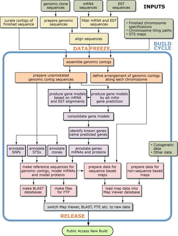
Figure 1The human genome assembly and annotation process
Tables
Table 1STS maps used for assembly or display
| Map type | Map | Contig assembly | Contig placement | Display |
|---|---|---|---|---|
| Genetic linkage | Genethon (20) | X | X | X |
| Genetic linkage | Marshfield (21) | X | X | X |
| Genetic linkage | Decode (22) | X | ||
| Radiation hybrid | GeneMap99-G3 (23, 24) | X | X | X |
| Radiation hybrid | GeneMap99-GB4 (23, 24) | X | X | X |
| Radiation hybrid | NCBI RH (25) | X | ||
| Radiation hybrid | Stanford G3 | X | X | X |
| Radiation hybrid | Stanford TNG (26) | X | X | |
| Radiation hybrid | Whitehead-RH | X | X | X |
| YAC | Whitehead-YAC | X | X | X |
Table 2Links from Map Viewer objects to other NCBI resources
| Map object | Linked NCBI resource | Resource description |
|---|---|---|
| Accession number | Entrez | Chapter 15 |
| Clone | Clone Registry |
http://www |
| Disease gene | OMIM | Chapter 7 |
| EST or mRNA | UniGene | Chapter 21 |
| Gene | LocusLink | Chapter 19 |
| Gene or transcript | Evidence Viewer | Chapter 20 |
| Gene or transcript | Model Maker | Chapter 20 |
| Gene | Human–mouse homology map |
http://www |
| STS | UniSTS |
http://www |
| Variation (SNP) | dbSNP | Chapter 5 |
Boxes
Box 1Annotation of other genomes
NCBI may assemble a genome prior to annotation, add annotations to a genome assembled elsewhere, or simply process an annotated genome to produce RefSeqs and maps for display in Map Viewer (Chapter 20).
The basic procedures used to annotate other eukaryotic genomes are essentially the same as those used to annotate the human genome. However, the overall process is adjusted to accommodate the different types of input data that are available for each organism. Genes can be annotated on any genome for which a significant number of mRNA, EST, or protein sequences are available. Other features, such as clones, STS markers, and SNPs, can also be annotated whenever the relevant data are available for an organism.
For example, genes and other features are placed on the mouse Whole Genome Shotgun (WGS) assembly from the Mouse Genome Sequencing Consortium (MGSC) by skipping the assembly steps used in the human process but following the annotation steps with relatively minor adjustments. A variation of the human process is also used to assemble and annotate genomic contigs from finished mouse clone sequences (see the Map Viewer display of the mouse genome).